Averaged dynamics and control for heat equations with random diffusion

By Jon Asier Bárcena Petisco, Enrique Zuazua

Background and motivation

Let us consider the random heat equation described by the following system:
$\begin{cases} y_t-\alpha \Delta y =f1_{G_0}, &\text{ in } (0,T)\times G,\\ y=0, & \text{ on } (0,T)\times \partial G,\\ y(0,\cdot)=y^0, & \text{ on } G, \end{cases}$

for $G$ a domain, $G_0\subset G$ a subdomain, $f$ a control, $y^0$ the initial configuration and $\alpha$ the diffusivity coefficient, which is a positive random variable with density function $\rho$ . We have that the averaged solution of (1) is given by:
$\tilde y(t,x;y^0,f):=\int_0^{+\infty} y(t,x;\alpha,y^0,f)\rho(\alpha)d\alpha.$ We want to determine if, given a positive random variable $\alpha$ and an initial configuration $y^0 \in L^2(G)$ , there is some $f \in L^2((0,T)\times G_0)$ such that $\tilde y(T,\cdot)=0$ .

In order to illustrate the effect of averaging in the dynamics, let us study the dynamics of (1) when $G=\mathbb R^d$ and $f=0$ . As averaging and the Fourier transform commute, we work on the Fourier transform of the fundamental solution of the heat equation, which is given by:
$\exp(-\alpha |\xi|^2t).$ Consequently, the Fourier transform of the average of the fundamental solutions is given by:
$\int_0^{+\infty} \exp (-\alpha |\xi|^2t)\rho(\alpha)d\alpha;$

i.e. the Laplace transform of $\rho$ evaluated in $|\xi|^2t$ . In particular, for $r\in(0,1)$ if $\rho(\alpha)\sim_{0^+} e^{-C\alpha^{-\frac{r}{1-r}}}$ we have that:

\int \exp (-\alpha |\xi|^2t)\rho(\alpha)d\alpha\sim \exp(-C|\xi|^{2r}t^r)

when $|\xi|^2t\to+\infty$ , which can be proved by the Laplace method. Thus, for those density functions the averaged dynamics in $\mathbb R^d$ has a fractional nature. As it is proved in [1],
for $G$ bounded this is also true and we have the usual controllability and observability results of fractional dynamics; that is, (2) implies that the averaged unique continuation is preserved,
but (2) preserves the null averaged observability if and only if $r>1/2$, being the threshold density functions those which satisfy:
$\rho(\alpha)\sim_{0^+} e^{-C\alpha^{-1}}.$

Some numerical simulations

Let us now illustrate the difference between several probability distributions for the diffusion through numerical simulations. For that, we recall that the optimal control is given by $\varphi(t,x;\phi)1_{G_0}$ , for $\varphi$ the averaged solution of
$\begin{cases} -\varphi_t-\alpha \Delta \varphi=0, &\text{ in } (0,T)\times G,\\ \varphi=0, & \text{ on } (0,T)\times\partial G,\\ \varphi(T,\cdot)=\phi, & \text{ on } G. \end{cases}$ and $\phi$ the state which minimizes the functional:
$J(\phi)= \frac{1}{2}\int_0^T\int_{G_0} \left|\int_0^{+\infty}\varphi(t,x;\alpha,\phi)\rho(\alpha)d\alpha\right|^2dxdt \\+\left\langle y^0, \int_0^{+\infty}\varphi(0;\alpha,\phi)\rho(\alpha)d\alpha\right\rangle.$ Due to the hardness of the numerical computations in higher dimensions and to get better illustrations we work in $d=1$ , and in particular in $G=(0,\pi)$ .
We also consider $G_0=(1,2), T=1$ and $y^0=\frac{1}{2}$ .
Moreover, to illustrate the difference between diffusivities inside and outside the null controllability regime, we consider $\rho=1_{(1,2)}$ , which is inside, and $\rho=1_{(0,1)}$ , which is outside.

In order to numerically implement this problem, we approximate it by minimizing $J$ in $V_M:=\langle e_i \rangle_{i=1}^M$ for $\{e_i\}$ the eigenfunctions of the Dirichlet Laplacian and for $M\in\{40,50,60\}$ . Since $V_M$ is a finite dimensional space, computing the minimum of $J$ is equivalent to solving numerically a linear system, which can be easily done by using any numerical computing environment (in our case MATLAB). We have the following illustrations:

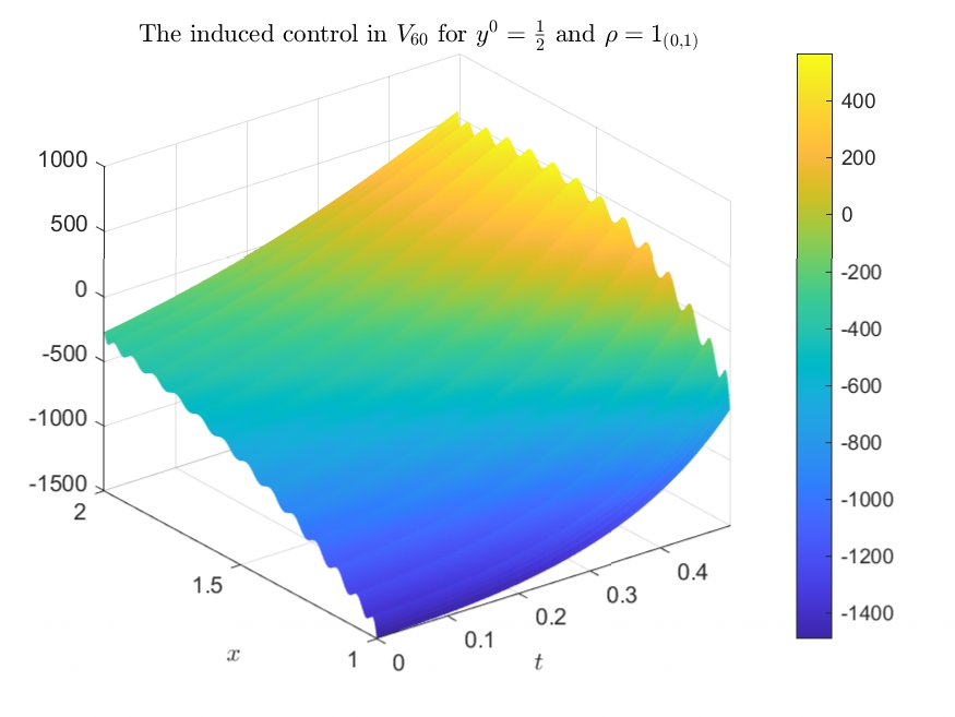
First, we illustrate in Figure 1 (resp. in Figure 2) the controls induced by the minimum of $J$ for $\rho=1_{(1,2)}$ (resp. for $\rho=1_{(0,1)}$ ).
For $\rho=1_{(1,2)}$ the sequence of controls converges, which is something that can be seen in an even more clear way when $t\in[0,1/2]$ . Of course, the closer the time is to $1$ , the more slowly the punctual values of the control converges pointwise with $M$ (and in $t=1$ it diverges), which is a well-known behaviour when controlling a parabolic dynamics (see, for instance, [2], [3] and [4]). However, for $\rho=1_{(0,1)}$ the sequence of controls diverges, which is something that we can appreciate in a more detailed way when $t\in[0,1/2]$ .

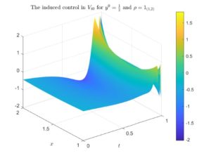
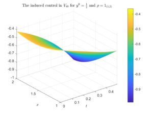
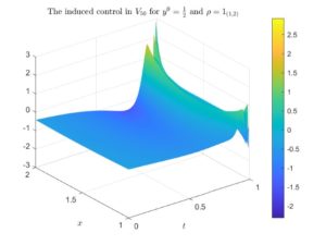
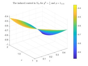
Figure 1. The optimal control for $\rho=1_{(1,2)}$ and $y^0=\frac{1}{2}$ induced by the minimum of the functional $J$ in $V_{40}, V_{50}$ and $V_{60}$ . In the left column we illustrate the whole controls, whereas in the right column we illustrate the controls with the time variable zoomed in $[0,1/2]$ .

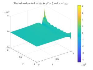
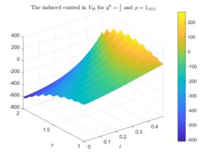
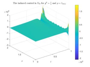
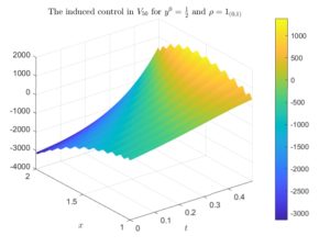
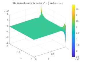
Figure 2. The optimal control for $\rho=1_{(0,1)}$ and $y^0=\frac{1}{2}$ induced by the minimum of the functional $J$ in $V_{40}$ , $V_{50}$ and $V_{60}$ . In the left column we illustrate the whole controls, whereas in the right column we illustrate the controls with the time variable zoomed in $[0,1/2]$ .

Next, we show in Figure 3 the canonical prolongation of the previously obtained controls to $t=0$ . Again, for $\rho=1_{(1,2)}$ we have a clear convergence, whereas for $\rho=1_{(0,1)}$ it diverges.

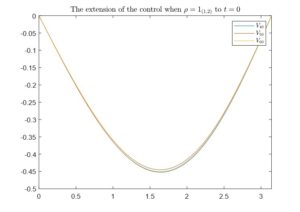
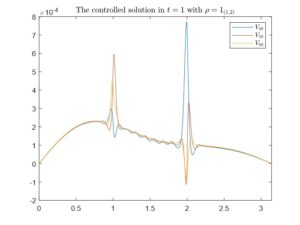
Figure 3. The natural extensions to $t=0$ of the controls induced by the minimum of the functional $J$ in $V_{40}, V_{50}$ and $V_{60}$ with $y^0=\frac{1}{2}$ . In the left figure we have considered $\rho=1_{(1,2)}$ and in the right one $\rho=1_{(0,1)}$ .

Finally, we illustrate in Figure 4 the state at $t=1$ of the respective solutions of the averaged heat equation with the previously obtained controls. For $\rho=1_{(1,2)}$ the solution converges smoothly to $0$ , whereas for $\rho=1_{(0,1)}$ the solution diverges.

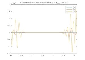
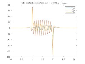
Figure 4. The state in time $t=1$ of the averaged solutions of the heat equation after applying the control induced by the minimum of $J$ in $V_{40}, V_{50}$ and $V_{60}$ with $y^0=\frac{1}{2}$ . In the left figure we have considered $\rho =1_{(1,2)}$ and in the right one $\rho=1_{(0,1)}$ .

References

[1] J. A. Bárcena-Petisco, E. Zuazua. Averaged dynamics and control for heat equations with random diffusion (2020)

[2] E. Fernández-Cara and A. Münch. Strong convergent approximations of null controls for the 1D heat equation. SeMA journal (2013), Vol. 61, No.1, pp.49-78

[3] R. Glowinski and J. L. Lions. Exact and approximate controllability for distributed parameter systems. Acta Numer. (1994), Vol. 1, pp. 269-378

[4] A. Münch and E. Zuazua. Numerical approximation of null controls for the heat equation: illposedness and remedies. Inverse Probl. (2010), Vol. 26, No. 8:085018