 Yanzhi Wu
1 Introduction
In this study, we consider an adaptive optimal output regulation problem for general linear systems. The purpose is to obtain both optimal feedback control gain and optimal feedforward control gain, which appear in the optimal controller and can help realize asymptotic and disturbance rejection. First, adaptive dynamic programming technique is used to solve the optimal feedback control gain. In reality, the problem of solving the optimal solution of a regulator equation can be transformed into a certain minimum norm problem in a Hilbert space. With the help of the projection theorem in the Hilbert space, the optimal solution of the regulator equation can be explicitly expressed.
2 Problem Formulation
In this study, the dynamics of the plant is described by
\begin{aligned} &\dot{x}=Ax+Bu+Ew,\\ &\dot{w}=\Gamma w,\\ &e=Cx+Du+Fw.\qquad (1) \end{aligned}
Let J_\Gamma={diag}(J_1,J_2,\cdots,J_l)\in \mathbb{R}^{q_m\times q_m} be the Jordan form corresponding to the matrix \Gamma in (1),
where
J_i=\begin{pmatrix}\lambda_i(\Gamma)&1&0&\cdots&0&0\\0&\lambda_i(\Gamma)&1&\cdots&0&0\\ \vdots&\vdots&\vdots&\vdots&\vdots&\vdots\\0&0&0&\cdots&\lambda_i(\Gamma)&1\\0&0&0&\cdots&0&\lambda_i(\Gamma)\end{pmatrix}\in \mathbb{R}^{q_{i}}, q_{1}+q_{2}+\cdots+q_{l}=q_m.
There must exist a nonsingular matrix T\in \mathbb{R}^{q_m\times q_m}, such that T^{-1}\Gamma T=J_{\Gamma}.
Denote w_1=T^{-1}w\in \mathbb{R}^{q_m}.
Considering the dynamics (1), one has
\dot{w}_1=J_\Gamma w_1. \qquad (2)
The linear output regulation problem is solved by designing a controller as follows
u=-Kx+Lw_1, \qquad (3)
where K is a feedback gain matrix, L=U+KX is a feedforward gain matrix to be designed,
and X, U satisfy the following regulator equation
\begin{aligned} XJ_\Gamma=&AX+BU+ET,\\ 0=&CX+DU+FT. \qquad (4) \end{aligned}
Let \hat{x}=x-Xw_1 and \hat{u}=u-Uw_1, then one has
\begin{aligned} \dot{\hat{x}} =&A\hat{x}+B\hat{u}, \qquad (5) \end{aligned}
\begin{aligned} e =&C\hat{x}+D\hat{u}. \qquad (6) \end{aligned}
The optimal output regulation problem is solved if and only if there exist an optimal feedback control gain K^* and an optimal feedforward control gain L^* such that K^* and L^* are respectively the minimizer of these two predefined performance indices.
To solve the optimal feedback control gain matrix K^*, we construct the following problem.
Problem 1
\begin{aligned} & \underset{(\hat{x},\hat{u})}{\text{minimize}} & & J(\hat{x},\hat{u})=\frac{1}{2}\int\limits_{t}^\infty \hat{x}^TQ\hat{x}+\hat{u}^TR\hat{u}d\tau \qquad (7) \\ & \text{subject to } & & (5), \end{aligned}
where Q=Q^T\geq 0, R=R^T>0, and (A,\sqrt{Q}) is observable.
Since L=U+KX, equally, L^*=U^*+K^*X^*, which means that the computation of L^* can be solved by the computation of U^*, K^* and X^*. With the optimal feedback gain matrix K^* from Problem 1, to solve the optimal feedforward control gain matrix L^*, Problem 2 is formally stated as follows.
Problem 2
\begin{aligned} & \underset{(X,U)}{\text{minimize}} & & \bar{J}(X,U)=\text{Tr}(X^TX+U^TU) \\ & \text{subject to } & & (4). \end{aligned}
3 Optimal Feedback Gain Matrix
In this section, a learning strategy is proposed, which can properly approximate the positive definite matrix P^* and the optimal feedback control gain K^*.
Let A_{j}=A-BK_{j}. Then the system (1) can be written as
\begin{aligned} \dot{x}&=A_{j}x+B(K_{j}x+u)+Ew. \qquad (8) \end{aligned}
Let Q_{j}=Q+(K_{j})^TRK_{j}. Then, one has
\begin{aligned} &x^T(t+\delta t)P_{j}x(t+\delta t)-x^T(t)P_{j}x(t)\\ =&\int_t^{t+\delta t}\Big[-x^TQ_{j}x+2\big(u+K_{j}x\big)^TRK_{j+1}x+2w^TE^TP_{j}x\Big]d\tau. \qquad (9) \end{aligned}
By Kronecker product representation, the expression in (9) can be further transformed as
\begin{aligned} x^TQ_{j}x&=(x^T\otimes x^T)\text{vec}(Q_{j}),\\ \big(u+K_{j}x\big)^TRK_{j+1}x&=\Big[\Big(x^T\otimes x^T\Big)\Big(I_{n}\otimes(K_{j}R)\Big)+\Big(x^T\otimes u^T\Big)\Big(I_{n}\otimes R\Big)\Big]\text{vec}(K_{j+1}),\\ w^TE^TP_{j}x&=(x^T\otimes w^T)\text{vec}(E^TP_{j}). \qquad (10) \end{aligned}
Furthermore, for positive integer s, considering (10), let
\begin{aligned} \delta_{xx}&=\Big[\text{vecv}(x(t_1))-\text{vecv}(x(t_0)), \cdots, \text{vecv}(x(t_s))-\text{vecv}(x(t_{s-1}))\Big]^T,\\ \Gamma_{xx}&=\Big[\int_{t_0}^{t_1}x\otimes xd\tau, \int_{t_1}^{t_2}x\otimes xd\tau, \cdots, \int_{t_{s-1}}^{t_s}x\otimes xd\tau\Big]^T,\\ \Gamma_{\bar{x}}&=\Big[\int_{t_0}^{t_1}\text{vecv}(x)d\tau,\cdots, \int_{t_{s-1}}^{t_s}\text{vecv}(x)d\tau\Big]^T,\\ \Gamma_{xu}&=\Big[\int_{t_0}^{t_1}x\otimes ud\tau, \int_{t_1}^{t_2}x\otimes ud\tau, \cdots, \int_{t_{s-1}}^{t_s}x\otimes ud\tau\Big]^T,\\ \Gamma_{xw}&=\Big[\int_{t_0}^{t_1}x\otimes wd\tau, \int_{t_1}^{t_2}x\otimes wd\tau, \cdots, \int_{t_{s-1}}^{t_s}x\otimes wd\tau\Big]^T, \qquad (11) \end{aligned}
where t_0 \lt t_1 \lt \cdots \lt t_s are positive integers. Considering (10) and (11), one can change (9) into the following form
\Psi_{j}\begin{pmatrix}\text{vecs}(P_j)\\ \text{vec}(K_{j+1})\\ \text{vec}(E^TP_{j})\end{pmatrix}=\Phi_{j}, \qquad (12)
where \Psi_{j}=\Big[\delta_{xx}, -2\Gamma_{xx}\Big(I_{n}\otimes \big((K_{j})^TR\big)\Big)-2\Gamma_{xu}(I_{n}\otimes R), -2\Gamma_{xw}\Big] and \Phi_{j}=-\Gamma_{xx}\text{vec}(Q_j).
Assume that \text{rank}\Big(\big[\Gamma_{xx}, \Gamma_{xu}, \Gamma_{xw}\big]\Big)=\frac{n(n+1)}{2}+(m+q_m)n holds, we note that \Psi_{j} is of full column rank. Therefore, the solution of (12) can be written as follows
\begin{pmatrix}\text{vecs}(P_j)\\ \text{vec}(K_{j+1})\\ \text{vec}(E^TP_{j})\end{pmatrix}=(\Psi_{j}^T\Psi_{j})^{-1}\Psi_{j}^T\Phi_{j}. \qquad (13)
It follows from (13) that both P_j and K_{j+1} can be calculated. We obtain that
B=P_{j}^{-1}K_{j+1}^TR, \qquad (14)
which can help compute the matrix B. Let j\leftarrow j+1. The stopping criterion is ||P_{j+1}-P_j||\leq \varepsilon, where \varepsilon is a small positive constant and j\geq 1.
4 Optimal Feedforward Gain Matrix
Having computed the approximation of the optimal feedback gain matrix K^* in the above subsection, our next step is to compute the approximation of the optimal feedforward gain matrix L^*, which is the solution of Problem 2.
To obtain the solutions of the regulator equation (4), we first rewrite (4) as the following form
\begin{aligned} &\begin{pmatrix}I_{n}&0_{n\times m}\\0_{p\times n}&0_{p\times m}\end{pmatrix}\begin{pmatrix}X\\U\end{pmatrix}J_\Gamma-\begin{pmatrix}A&B\\C&D\end{pmatrix}\begin{pmatrix}X\\U\end{pmatrix}=\begin{pmatrix}ET\\FT\end{pmatrix}. \qquad (15) \end{aligned}
Furthermore, (15) can be rewritten as the following standard linear equation by using the properties of the Kronecker product
\bar{\mathcal{A}}\bar{z}=b, \qquad (16)
where \bar{\mathcal{A}}=J_\Gamma^T\otimes \mathcal{E} -I_q\otimes\bar{A}\in \mathbb{R}^{\Big(q_m(n+p)\Big)\times \Big(q_m(n+m)\Big)}, \mathcal{E}=\begin{pmatrix}I_{n}&0_{n\times m}\\0_{p\times n}&0_{p\times m}\end{pmatrix}, \bar{A}=\begin{pmatrix}A&B\\C&D\end{pmatrix}, \bar{z}=\text{vec}\begin{pmatrix}X\\U\end{pmatrix}\in \mathbb{R}^{q_m(n+m)}, and b=\text{vec}\begin{pmatrix}ET\\FT\end{pmatrix}\in \mathbb{R}^{q_m(n+p)}. Therefore, the matrix \bar{\mathcal{A}}=\text{blockdiag}(\hat{\mathcal{A}}_{1},\hat{\mathcal{A}}_{2},\cdots,\hat{\mathcal{A}}_{l}) is a block diagonal matrix with its jth (j=1,2,\cdots,l) block diagonal element as
\hat{\mathcal{A}}_{j}=\begin{pmatrix}\lambda_j(\Gamma)\mathcal{E}-\bar{A}&0&\cdots&0&0\\ \mathcal{E}&\lambda_j(\Gamma)\mathcal{E}-\bar{A}&\cdots&0&0\\ \vdots&\vdots&\vdots&\vdots&\vdots\\0&0&\cdots&\mathcal{E}&\lambda_j(\Gamma)\mathcal{E}-\bar{A}\end{pmatrix}, \qquad (17)
where \hat{\mathcal{A}}_{j}\in \mathbb{R}^{\Big(q_j(n+p)\Big)\times \Big(q_j(n+m)\Big)}.
The matrix \bar{\mathcal{A}} is of full row rank. Let \bar{\mathcal{A}}_{j} denotes the jth row of the matrix \bar{\mathcal{A}} for j=1,2,\cdots,(n+p)q_m.
Obviously, \bar{\mathcal{A}}_{j} and \bar{\mathcal{A}}_{k} for j,k=1,2,\cdots,(n+p)q_m, j\neq k are independent vectors, and the condition (16) can be understood as
(\bar{\mathcal{A}}_{1},\bar{z})=b_{1}, \cdots, (\bar{\mathcal{A}}_{(n+p)q_m},\bar{z})=b_{(n+p)q_m}, where b_{j} denotes the jth element of the column vector b for j=1,2,\cdots,(n+p)q_m.
The detailed expression of the optimal solution of (4) can be written as
\bar{z}=\sum\limits_{j=1}^{(n+p)q_m}\alpha_{j}\bar{\mathcal{A}}_{j}, \qquad (18)
which has the minimum form and these coefficients \alpha_1,\cdots,\alpha_{(n+p)q_m} satisfy
\begin{aligned} \langle \bar{\mathcal{A}}_{1},\bar{\mathcal{A}}_{1}\rangle\alpha_{1}+\cdots+\langle \bar{\mathcal{A}}_{(n+p)q_m},\bar{\mathcal{A}}_{1}\rangle\alpha_{(n+p)q_m}=&b_{1},\\ \cdots\quad\quad\cdots\quad\quad\cdots\quad\quad \cdots\quad\quad \cdots&\\ \langle \bar{\mathcal{A}}_{1},\bar{\mathcal{A}}_{(n+p)q_m}\rangle\alpha_{1}+\cdots+\langle \bar{\mathcal{A}}_{(n+p)q_m},\bar{\mathcal{A}}_{(n+p)q_m}\rangle\alpha_{(n+p)q_m}=&b_{(n+p)q_m}. \qquad (19) \end{aligned}
Denote
\hat{\mathcal{A}}=\begin{pmatrix}\langle \bar{\mathcal{A}}_{1},\bar{\mathcal{A}}_{1}\rangle&\cdots&\langle \bar{\mathcal{A}}_{(n+p)q_m},\bar{\mathcal{A}}_{1}\rangle\\
\vdots&\vdots&\vdots\\ \langle \bar{\mathcal{A}}_{1},\bar{\mathcal{A}}_{(n+p)q_m}\rangle&\cdots&\langle \bar{\mathcal{A}}_{(n+p)q_m},\bar{\mathcal{A}}_{(n+p)q_m}\rangle\end{pmatrix}.
\hat{\mathcal{A}} is a positive definite matrix. Denote \alpha={col}(\alpha_{1},\alpha_{2},\cdots,\alpha_{(n+p)q_m}). Then one has \alpha=\hat{\mathcal{A}}^{-1}b.
Based on the variable \alpha, we compute the optimal solution of Problem 2, \begin{pmatrix}X^*\\ U^*\end{pmatrix}, and then compute the approximated optimal feedforward control gain L_j^*=U^*+K_j^*X^*.
5 Simulation
In this section, a simulation example is given to prove the correctness of our theory results.
The dynamics is given by (1), where A=\begin{pmatrix}0&1&0\\0&0&1\\0&0&0\end{pmatrix}, B=\begin{pmatrix}0\\0\\1\end{pmatrix}, C=\begin{pmatrix}1&0&0\end{pmatrix}, D=1.
F=\begin{pmatrix}5\sqrt{3}&5&0&0\end{pmatrix}. The system matrix of the exosystem is \Gamma=\begin{pmatrix}0&-2\pi&0&0\\2\pi&0&0&0\\0&0&0&-3\pi\\0&0&3\pi&0\end{pmatrix} and w(0)={col}(1,0,1,0). Let Q=I_3 and R=1. The stopping criterion ||P_{j}-P_{j-1}||\leq 0.001 is satisfied after six iterations, the approximated optimal feedback gain K_j^* is K_j^*=\begin{pmatrix}1.0076&2.3614&2.4362\end{pmatrix}, and the approxiate optimal feedforward control gain L_j^* is L_j^*=\begin{pmatrix}-4.6071 + 5.6847i&-4.6071 - 5.6847i&0&0\end{pmatrix}. The eigenvalues of the matrix A-BK_j^*, namely, -0.6480 + 0.6810i, -0.6480 - 0.6810i, -1.1402 + 0.0000i, all have negative real parts.
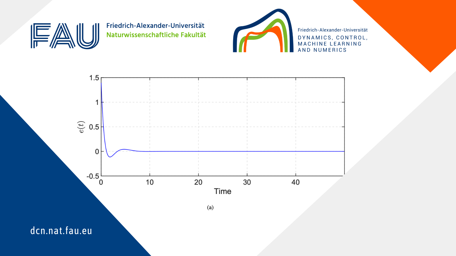
Figure 1 shows the evolution of the regulated output.
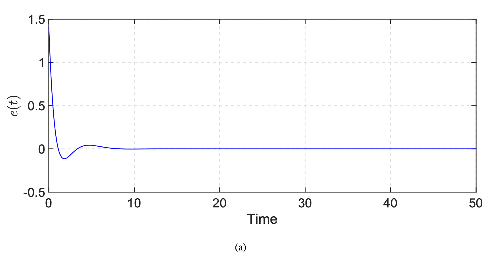
Figure 1. Evolution of the regulated output e(t)
6 Conclusions
In this study, we have addressed the adaptive optimal output regulation problem for general linear systems. To obtain the optimal controller, both optimal feedback control gain matrix and the optimal feedforward control gain matrix are computed by using the adaptive dynamic programming, output regulation theory and the projection theorem in the Hilbert space. Our further work will focus on the optimal output regulation problem for nonlinear systems.
|| Go to the Math & Research main page