How to steer a fleet of agents by controlling only a few: A mean-field approach

How to steer a fleet of agents by controlling only a
few: a mean-field approach

1 Introduction

The challenge of controlling large systems of interacting agents has garnered significant attention in recent years. Applications of such problems include crowd evacuations, achieving consensus within a large group, and traffic flow control. In many scenarios, controlling each individual agent is either prohibitively expensive or infeasible due to the problem constraints. A practical solution involves achieving the desired objectives by controlling only a small subset of agents. A classical example is a shepherd steering a flock of sheep using just a few dogs.

Even in this simplified setting, which reduces the number of parameters to learn, the problem remains computationally challenging, especially when the number of noncontrollable agents is large. One approach that has been widely adopted to simplify the study of large multi-agent systems is the mean field approach. In this method, agents are approximated by a continuum, and their dynamics are described by a partial differential equation (PDE).

The specific model in $\R^d$ we consider consists of a non-local continuity equation coupled with a controlled ordinary differential equation [3]:

$\begin{cases} \partial_t\mu(t)+\mathrm{div}\bigl(F[\mu(t)](\cdot,\bold{y}(t))\mu(t)\bigr) = 0,\\ \dot{y}^m(t)=u^m(t), \hspace{1.5cm} m=1,\dots, M, \hspace{1cm}(1) \end{cases}$

where $\mu(t)\in\mathcal{P}(\R^d)$ represents the distribution of non-controllable agents at time $t \in [0,T]$ , and, for $m = 1, \dots, M, y^m$ denotes the position of the $m$ -th controllable agent, and $u^m$ is its control law. The interaction term $F$ models the influence of both the agent distribution and the controllable agents. A typical choice for $F$ is

$F[\mu](x,y) = \int_{\mathbb{R}^d} K(x - \zeta) \, d\mu(\zeta) + \frac{1}{M}\sum_{m=1}^M f(x - y^m),$

where $y=(y^1,...,y^M)$ and $K$ and $f$ describe the interaction kernels.
Associated with this dynamical model, we consider the following optimal control problem

$\inf_u \psi\bigl(\boldsymbol{\mu}(\mu_0, y_0, u; T)\bigr), \hspace{1cm} (OCP)$

where $t \mapsto \boldsymbol{\mu}(\mu_0, y_0, u; t)$ is the solution of (1) with initial conditions $\mu_0 \in \mathcal{P}_c(\mathbb{R}^d)$ and $y_0 = (y_0^1, \dots, y_0^M)\in\R^{dM}$ , control law $u = (u^1, \dots, u^M)$ , and the final time $T>0$ is fixed. We assume $u$ to vary in the set of admissible controls $\mathcal{U}\coloneqq L^\infty([0,T],U^M)$ where $U\subseteq \R^d$ is a compact set. Common choices for the terminal cost $\psi$ include expected values and the squared Wasserstein distance from a reference measure $\hat{\mu}$ :

$\psi(\mu) = \int_{\mathbb{R}^d} \alpha(\xi)\, d\mu(\xi) \quad \text{or} \quad \psi(\mu) = \frac{1}{2} W_2(\mu, \hat{\mu})^2,$

where $\alpha\colon \R^d\to\R$ is a sufficiently regular function. The minimization of the Wasserstein distance provides a means to steer the system toward a desired configuration. For instance, it can achieve a state where the non-controllable agents are uniformly distributed, a challenging task when approached from a finite-dimensional perspective.
The objective of this post is to present, in an accessible manner, key results related to (OCP) and to demonstrate, through simulations, the effectiveness of the mean-field approach.

2 Necessary Optimality Conditions

Under standard Lipschitz regularity assumptions on the vector field $F$ , it is possible to establish existence and uniqueness of solutions of (1) analogously to the well-known Cauchy-Lipschitz theorem for ODEs. Here solutions of the continuity equation are understood in the distributional sense. Furthermore, the solution depends continuously on initial conditions and controls (considering the weak-* topology in $L^\infty$ ). This observation is key to proving the following result:

Theorem 2.1.
If $\psi$ is weakly lower semicontinuous, then (OCP) admits solutions.
Proof.
The control set $\mathcal{U}$ is weakly-* compact in $L^\infty$ due to its boundedness. Therefore, by the Weierstrass theorem and the continuous dependence of solutions on the control laws, the existence of an optimal control is guaranteed.

With this result established, we can now turn our attention to deriving first-order optimality conditions. Specifically, we state a Pontryagin minimum principle, a wellknown tool in optimal control theory, for (OCP), but before we present its classical finite-dimensional version [2, Theorem 6.1.1].

Theorem 2.2.
If $u^*$ is an optimal control for

$\inf_u \psi(x(x_0,u;T))$

with constraints given by the ordinary differential equation

$\dot{x}(t)= g(x(t)) + u(t)\hspace{1.5cm} x(t)\in\R^d$

and $x^*$ is the corresponding optimal state trajectory, then there exists a co-state $p^*$ which is the solution of the adjoint linearized equation

$\dot{p}^*(t)=-p^*(t)^TD_xg(x^*(t),u^*(t))\hspace{1.2cm} p^*(T) = \nabla_x\psi(x^*(x_0,u^*;T))$

and such that the following optimality condition

$p^*(t)\cdot u^*(t)=\min_{\omega\in U} p^*(t)\cdot \omega$

for almost every $t\in [0,T]$ .

The mean-field version of this theorem is as follows. Similar results appear in [2] and [1].

Theorem 2.3.(Informal Pontryagin Minimum Principle for (OCP)).
If $u^*$ is an optimal control for (OCP) and $(\boldsymbol{\mu}^*, y^*)$ is the corresponding optimal solution of (1), then there exists a curve of probability measures $\boldsymbol{\rho}^*$ and a curve $\bold{q}^*$ in $\R^{dM}$ such that $(\boldsymbol{\rho}^*, \bold{q}^*)$ solves the adjoint Wasserstein linearized system associated with (1) with terminal condition:

$\boldsymbol{\rho}^*(T) = \nabla_\mu \psi[\boldsymbol{\mu}^*(T)]_*\boldsymbol{\mu}^*(T)\hspace{1.2 cm}\text{and}\hspace{1.2cm}\bold{q}^*(T)=0$

and satisfying the optimality conditions:

$\bold{q}^*(t)\cdot u^*(t)=\min_{\omega^1,...,\omega^M\in U} \bold{q}^*(t)\cdot (\omega^1,...,\omega^M)\quad \text{for almost every } t \in [0,T].$

In the theorem above, $\nabla_\mu \psi[\boldsymbol{\mu}^*(T)]\in L^2(\R^d,\R^d;\boldsymbol{\mu}^*(T))$ represents the Wasserstein gradient of $\psi$ at $\boldsymbol{\mu}^*(T)$ and $_*$ is the pushforward operator. For further details on Wasserstein calculus, we refer readers to [4]. This result closely parallels its classical counterpart: the distribution $\boldsymbol{\rho}^*$ can be interpreted as the distribution of the non-controllable co-states, while $\bold{q}^*$ represents the vector of co-states for the controllable agents. Additionally, the terminal condition corresponds to the gradient of the loss function evaluated at the final optimal state distribution.

3 Numerical Simulations

As with classical optimal control problems, in the Wasserstein setting of probability measures, the adjoint equation provides a practical tool for computing gradients of the loss function with respect to the control.

Theorem 3.1.
The following equality holds:

$\frac{d}{du} \psi\bigl(\boldsymbol{\mu}(\mu_0,y_0,u; T)\bigr)\biggr\rvert_{u = \hat{u}} = \bold{q}(\mu_0,y_0,\hat{u};\cdot),$

where $t\mapsto \mathbf{q}(\mu_0,y_0,\hat{u};t)$ is the co-state associated with the controllable agents subject to the control $\hat{u}$ with initial conditions $\mu_0$ and $y_0$ .
Using this result, gradient-based methods such as gradient descent can be employed to find solutions. Specifically, a sequence of controls can be generated as follows

$u_{k+1} = u_k - \eta \frac{d}{du} \psi \bigl(\boldsymbol{\mu}(\mu_0,y_0,u_k; T)\bigr) \biggr\rvert_{u = u_k},$

where $\eta>0$ is the learning rate. The theorem implies that to compute the gradient of the loss at a point $u^*$ , one must first solve the forward equation for the given control, followed by a backward pass to solve the adjoint equation and obtain the co-state $\mathbf{q}$ .
In the following we show some numerical simulations obtained using these methods, demonstrating their practical applicability. Even if the lack of convexity of the problem neglects the possibility to guarantee convergence to global minimizers, satisfactory results are obtained.

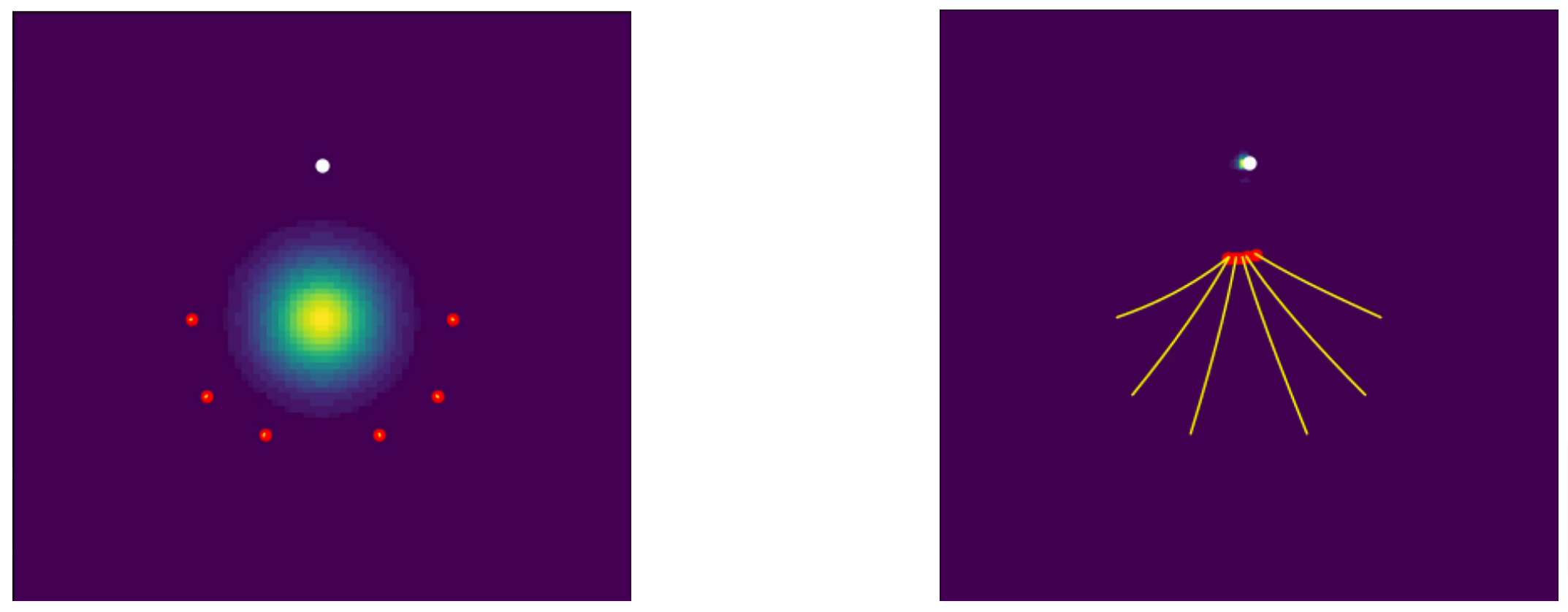
Figure 1. Six dogs (red dots) steer a Gaussian distribution toward the target (white dot). On the left is the initial configuration, while on the right is the final one. Orange lines represent the dogs’ trajectories.

References

[1] M. Bongini, M. Fornasier, F. Rossi, and F. Solombrino (2017) Mean-field pontryagin maximum principle. J. Optim. Theory Appl., Vol. 175, pp. 1–38
[2] M. Fornasier and F. Solombrino (2014) Mean-field optimal control. ESAIM: COCV, Vol. 20, No. 4, pp. 1123–1152
[3] Massimo Fornasier, Benedetto Piccoli, and Francesco Rossi (2014) Mean-field sparse optimal control. Philosophical Transactions of the Royal Society A: Mathematical, Phys. Eng. Sci., Vol. 372, No. 2028, 20130400
[4] N. Lanzetti, S. Bolognani, and F. Dörfler (2022) First-order conditions for optimization in the wasserstein space. arXiv preprint