Aggregation of Finite-Valued Networks Based on Bisimulation

1 Backgrounds

The finite-valued networks are important models in complex system engineering. These systems are characterized as multi-agent dynamics with nodes taking values in finite sets endowed with operators. The study of finite-valued functions and systems can be traced back to finite automata [6], encryption-decryption in cryptography [1], and Boolean networks in theoretical biology [3].
In the analysis and design of finite-valued networks, the commonly used methods consists of symbolic approach and the algebraic state-space representation (ASSR). The former is not easy for deriving uniform expression while the latter suffers from high computational complexity [2].
In our work, we present an aggregation method for the ASSR based on bisimulation, to reduce the model dimensionality.

2 Problem Formulation

A $k$ -valued control network is a multi-agent system of $n$ nodes evolving over a finite-valued set ${\cal D}_k:=\{1,\cdots,k\}$ :

$\begin{array}{l} x_i(t+1)=f_i(x_1(t),\cdots,x_n(t), u_1(t),\cdots,u_m(t)), \quad i=1,\cdots,n,\\ y_j(t)=h_j(x_1(t),\cdots,x_n(t)),\quad j=1,\cdots,p, \qquad (2.1) \end{array}$

where $x_i(t)\in {\cal D}_k$ , $i=1,\ldots,n$ are states, $u_s(t)\in {\cal D}_k$ , $s=1,\ldots,m$ are inputs (or controls),
$y_j(t)\in {\cal D}_k$ , $j=1,\ldots,p$ are outputs (or observations), $f_i:{\cal D}_k^n\times {\cal D}_k^m \rarr {\cal D}_k$ , $i=1,\ldots,n$ are state updating functions, $h_j:{\cal D}_k^n \rarr {\cal D}_k$ , $j=1,\ldots,p$ are output functions.

By identifying $i$ as a logical vector $(0,\cdots,0,1,0,\cdots,0)^{\mathrm{T}}$ with the $i$ -th entry nonzero, the system (2.1) can be converted into the following algebraic state space representation

$\begin{cases} x(t+1)=L(u(t)\otimes x(t)),\\ y(t)=Hx(t), \qquad (2.2) \\ \end{cases}$

where $L\in {\cal L}_{k^n\times k^{n+m}}$ , $H\in {\cal L}_{k^p\times k^n}$ are logical matrices, called the structure matrices.

One sees that the dimension of system (2.2) grows exponentially with the number of the nodes. In what follows we shall reduce it using the observational equivalence.
The main concept in our aggregation approach, the so-called bisimulation, is based on the quotient dynamics of transition systems.

Definition 2.1
Consider a transition system $T=(X,U,\Sigma,O,h)$ , where $X$ is the set of states, $U$ is the set of inputs (controls or actions), $\Sigma:X\times U \rarr 2^X$ is a transition mapping, $O$ is the set of observations, $h:X\rarr O$ is the observation mapping.
The tuple $T/\sim :=(X/\sim,U,\Sigma_{\sim},O,h_{\sim})$ is called the quotient system of $T$ under observational equivalence, where
(i) $X/\sim=\{x/\sim\;|\; x\in X\}$ is the set of (observational) equivalence classes.
(ii) $U$ is the (original) set of inputs.
(iii) $\Sigma_{\sim}:X/\sim \times U \rarr 2^{X/\sim}$ , defined as follows. Suppose $X_i,X_j\in X/\sim$ , then $X_j\in \Sigma_{\sim}(X_i,u)$ if and only if, $\exists x_i\in \mathrm{con}(X_i),x_j\in \mathrm{con}(X_j)$ , s.t. $x_j\in \Sigma(x_i,u)$ .
(iv) $O$ is the (original) set of observations.
(v) $h_{\sim}:X/\sim \rarr O$ , defined as follows: $h_{\sim}(X_i):=h(x_i)$ , $x_i\in \mathrm{con}(X_i)$ .

Let $x_1\sim x_2$ denote the equivalence relation that $x_1$ , $x_2$ have identical observations. If for any $u\in U$ and $x_1'\in \Sigma(x_1,u)$ there exists $x_2'\in \Sigma(x_2,u)$ such that $x_1'\sim x_2'$ , then we say $x_1\approx x_2$ . If for any $x_1\sim x_2$ we have $x_1\approx x_2$ , then $T/\sim$ is called a bisimulation of $T$ , denoted by $T/\approx$ .

Intuitively, the bisimulation indicates that the input-output relation of one transition system can be fully recovered from that of another system, and vice versa, depicted as in Figure 1.

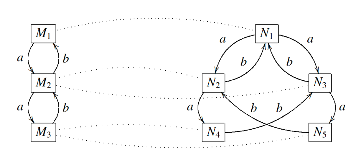
Figure 1. Bisimluation between finite transition systems [5]

3 Main Results

We propose an aggregation algorithm for system (2.1) (correspondingly, (2.2)), based on the observational equivalence and bisimulation relation derived from the equivalence.

Consider a network $\Sigma$ with network graph $(N,E)$ , where $N=\{x_1,x_2,\cdots,x_n\}$ .
Let $A=\{x_{a_1},\cdots,x_{a_{n_A}}\}\subset N$ , where $\{a_1,a_2,\cdots,a_{n_A}\}\subset [1,n]$ . Let $A^c:=N\backslash A$ . If $(x_i,x_j)\in E$ , $x_i\in A^c$ , $x_j\in A$ , then $x_i$ is called a formal input of $A$ . If $(x_i,x_j)\in E$ , $x_i\in A$ , $x_j\in A^c$ , then $x_i$ is called a formal output of $A$ .
$A$ is called an aggregatable block if there is no $(x_i,x_j)\in E$ such that $x_i$ is a formal input and $x_j$ is a formal output.

Proposition 3.1
Let $A\subset N$ be an aggregatable block of the network $\Sigma$ . Suppose the dynamics of the transition system $\Sigma_A$ with formal inputs $v_1,\cdots,v_{\alpha}\in N\backslash{A}$ and formal outputs $y_1,\cdots,y_{\beta}\in A$ has structure matrices of dynamics and observation $L_A$ , $H_A$ respectively, then its quotient system under output equivalence with respect to the formal outputs, denoted by $\Sigma_A/\sim$ , is a bisimulation if and only if

$H\times_{\cal B} L_A\times_{\cal B} (I_m\otimes H^\mathrm{T})\in{\cal L}_{k^s\times k^s}, \qquad (3.1)$

where $H$ is the structure matrix of the function $\otimes_{i=1}^rx_i \rarr \otimes_{j=1}^{s}x_{i_j}$ , and $\times_{\cal B}$ is the Boolean product.
The quotient system has the dynamics as

$y(t+1)=\tilde{L}_A(u(t)\otimes v(t)\otimes y(t)), \qquad (3.2)$

where $\tilde{L}_A=H_A\times_{{\cal B}} L_A\times_{{\cal B}} (I_{k^{m+ \alpha}}\otimes H^{T}_A)\in {\cal B}_{\xi\times \eta}$ , $\xi:=k^{\beta}$ , $\eta:=k^{m+\alpha+\beta}$ , $v:=\otimes_{i=1}^{\alpha}v_i$ , $y:=\otimes_{j=1}^{\beta}y_j$ , $u:=\otimes_{\ell=1}^{m}u_{\ell}$ . If $\Sigma_A/\!\sim=\Sigma_A/\!\approx$ is a bisimulation, then the aggregation does not affect the dynamics of the overall system.

The above criterion provides a way of deriving the dynamics of aggregatable blocks and replacing the subnetworks with lower-dimensional equivalences.
Finally, when the aggregation does not provide a bisimulation, we propose the following algorithm to transform the aggregatable block into a finite Markov chain of lower dimension.
We propose the following aggregation algorithm:
Data: $k$ -valued network $\Sigma$ with network graph $(N,E)$ .
• Step 1: Partition the networks according to the balancing principle (aggregate the states which are neither controllable nor observable), choose $A\subset N$ an aggregatable block with transition dynamics $\Sigma_A$ and structure matrices $L_A$ , $H_A$ .
• Step 2: Aggregate $A$ following the observational equivalence, replacing the Boolean product in (3.1) with conventional product, set $M_A:=H_AL_A(I_{k^{m+\a}}\otimes H^\mathrm{T}_A)$ , and verify if it is a logical matrix.
• Step 3: Calculate the approximate bisimulation when the aggregated subnetworks are not exact. Suppose $M_A=(m_{i,j})\in {\cal M}_{\xi\times \eta}$ , denote
$m_j:=\sum_{i=1}^{\xi}m_{i,j}$ , $j\in [1,\eta]$ . Construct a Markov chain with the same formal inputs and formal outputs as $\Sigma_A/\sim$ and its dynamics in ASSR is

$y(t+1)=M^{i_1,i_2,\cdots,i_{\eta}}(u(t)\otimes v(t)\otimes y(t)),\quad i_j\in [1,\xi],\;j\in [1,\eta],$

where each $M^{i_1,i_2,\cdots,i_{\eta}}$ takes the value $\delta_{\xi}[i_1,i_2,\cdots,i_{\eta}]$ with probability $p_{i_1,i_2,\cdots,i_{\eta}}=\prod_{j=1}^\eta\frac{m_{i_j,j}}{m_j}$ .

4 An Example

We consider the T cell receptor kinetics modeled in [4] as an example. The following is taken from [7] with the physical meaning of the nodes omitted.

The dynamics of the network of T cell receptor kinetics with $37$ nodes and $3$ controls, all of binary values, shown in Figure 2, is described in the following equations, where $x_i(*)=f(x_{j_1},\cdots,x_{j_i})$ is a shortened expression of $x_i(t+1)=f(x_{j_1}(t),\cdots,x_{j_i}(t))$ , while $f_i$ is a logical function generated from basic operators (conjunction, disjunction, negation), $i=1,\cdots,37$ .

$\begin{array}{l} x_1(*)=x_9\wedge x_{18},~x_2(*)=x_{14},~x_3(*)=x_2,~x_4(*)=x_{37},\\ x_5(*)=x_6,~x_6(*)=x_{32},~x_7(*)=x_{25},~x_8(*)=x_{21},\\ x_9(*)=x_8,~x_{10}(*)=(x_{20}\wedge u_2)\vee(x_{35}\wedge u_2),\\ x_{11}(*)=x_{19},~x_{12}(*)=x_{19},~x_{13}(*)=x_{24},~x_{14}(*)=x_{25},\\ x_{15}(*)=x_{34}\wedge x_{37},~x_{16}(*)=\overline{x_{13}}, ~x_{17}(*)=x_{33},\\ x_{18}(*)=x_{17}, ~x_{19}(*)=x_{37},~x_{20}(*)=\overline{x_{26}}\wedge u_1\wedge u_2,\\ x_{21}(*)=x_{28},~x_{22}(*)=x_{3}, ~x_{23}(*)=\overline{x_{16}},~x_{24}(*)=x_{7},\\ x_{25}(*)=(x_{15}\wedge x_{27}\wedge x_{34}\wedge x_{37})\vee(x_{27}\wedge x_{31}\wedge x_{34}\wedge x_{37}),\\ x_{26}(*)=x_{10}\vee\overline{x_{35}},~x_{27}(*)=x_{19},~x_{28}(*)=x_{29},\\ x_{29}(*)=x_{12}\vee x_{14},~x_{30}(*)=x_{7}\wedge x_{13},~x_{31}(*)=x_{20},\\ x_{32}(*)=x_{8},~x_{33}(*)=x_{24},~x_{34}(*)=x_{11},~x_{35}(*)=\overline{x_{4}}\wedge u_3,\\ x_{36}(*)=x_{10}\vee (x_{20}\wedge x_{35}), ~x_{37}(*)=\overline{x_{4}}\wedge x_{20}\wedge x_{36}. \end{array}$

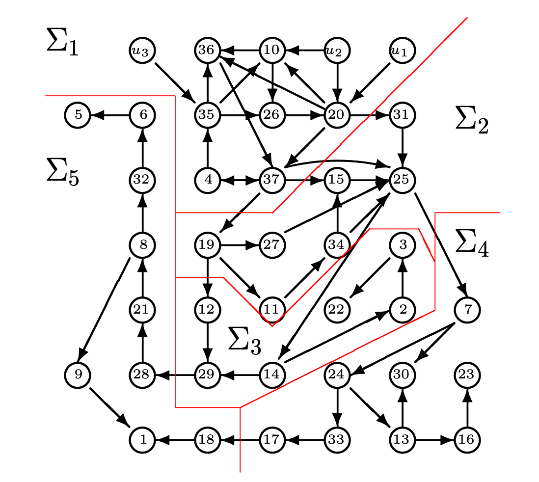
Figure 2. T cell receptor kinetics

It is natural to consider the nodes with zero out-degree as observers. So we have $y_1=x_1$ , $y_2=x_5$ , $y_3=x_{22}$ , $y_4=x_{23}$ , $y_5=x_{30}$ .
Then the network is divided into 5 blocks. We will use simulation to aggregate them.

Each block $\Sigma_i$ is characterized by $z^i(t+1)=L_iv^i(t)z^i(t)$ , $q^i(t)=H_iz^i(t)$ , $i=1$ , $2$ , $\cdots$ , $5$ , where $z^i$ is the algebraic from of the state in the corresponding subnetwork $\Sigma_i$ , and $v^i$ and $q^i$ are the formal inputs and formal outputs of the block, respectively, while $H_i$ , $L_i$ are the structure matrices.

We will use $\Sigma_2$ as an example to illustrate the approximate aggregation to a block.
Within $\Sigma_2$ , rename the variables as follows: $z_1=x_{11}$ , $z_2=x_{15}$ , $z_3=x_{19}$ , $z_4=x_{25}$ , $z_5=x_{27}$ , $z_6=x_{31}$ , $z_7=x_{34}$ ; $v_1=x_{20}$ , $v_2=x_{37}$ ; $q_1=x_{19}$ , $q_2=x_{25}$ , where $v_1$ , $v_2$ are block inputs, $q_1$ , $q_2$ are block outputs.

Then from the structure matrices of the block dynamics as $L_2\in {\cal L}_{128\times 512}$ ,
$H_2\in {\cal L}_{4\times 128}$ ,
Following the aggregation algorithm,
we normalize the matrix $H_2L_2(I_4\otimes H_2^\mathrm{T}):=T^2$ , then
the probabilistic approximation of $\Sigma_2$ is obtained by updating $T^2$ with

$T^2=\left[ \begin{array}{cccccccccccccccc} \frac{1}{8}&\frac{1}{8}&\frac{1}{8}&\frac{1}{8}&0&0&0&0&\frac{1}{8}&\frac{1}{8}&\frac{1}{8}&\frac{1}{8}&0&0&0&0\\ \frac{7}{8}&\frac{7}{8}&\frac{7}{8}&\frac{7}{8}&0&0&0&0&\frac{7}{8}&\frac{7}{8}&\frac{7}{8}&\frac{7}{8}&0&0&0&0\\ 0& 0& 0& 0&0&0&0&0& 0& 0& 0& 0&0&0&0&0\\ 0& 0& 0& 0&1&1&1&1& 0& 0& 0& 0&1&1&1&1\\ \end{array} \right].$

Similarly, the ASSR is obtained for the systems $\Sigma_1$ , $\Sigma_3$ , $\Sigma_4$ and $\Sigma_5$ . Summarizing these dynamics of blocks, an overall aggregated simulation for T cell is shown in Figure 3, where $z^1_1=x_{20}$ , $z^1_2=x_{37}$ , $z^2_1=x_{19}$ , $z^2_2=x_{25}$ , $z^3_1=x_{22}$ , $z^3_2=x_{29}$ , $z^4_1=x_{23}$ , $z^4_2=x_{30}$ , $z^4_3=x_{17}$ , $z^5_1=x_{1}$ , $z^5_2=x_{5}$ .

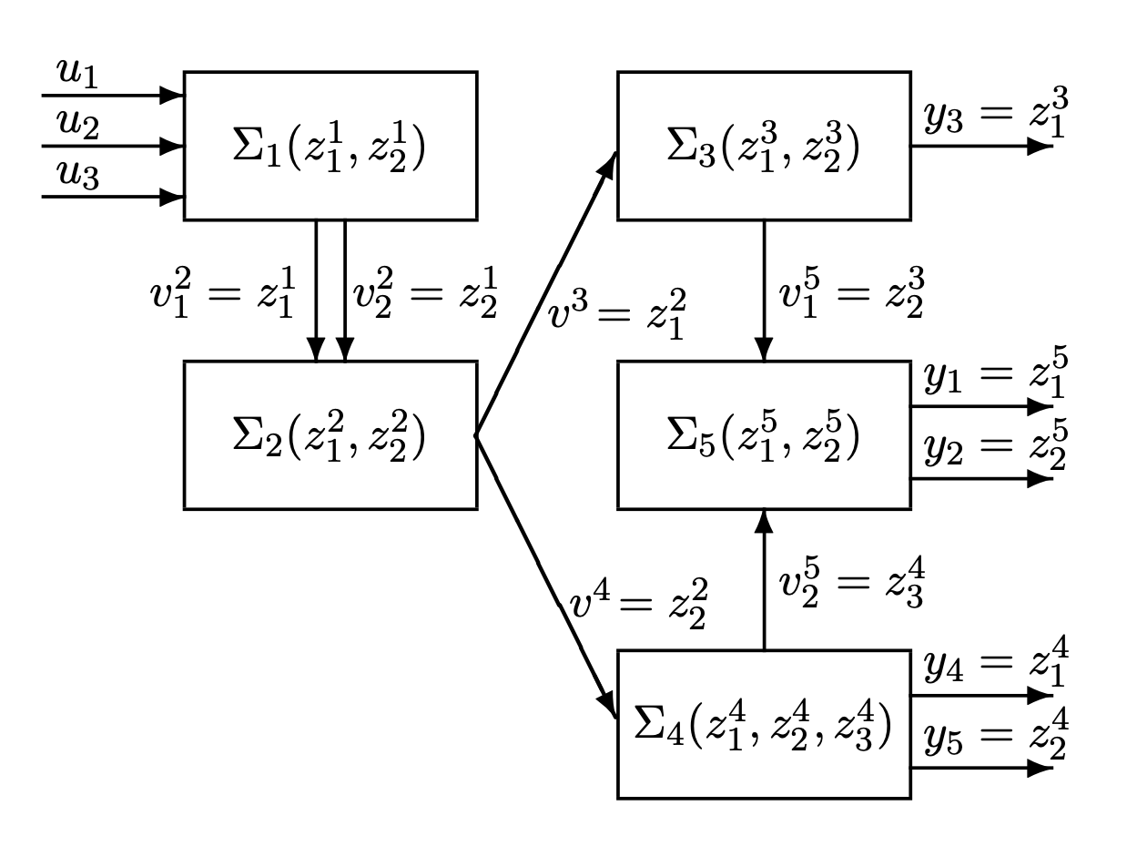
Figure 3. Aggregated bisimulation of T Cell receptor kinetics

This aggregated system has only $11$ state nodes and $3$ controls, which significantly simplifies the original model. Of course, the transition form of this quotient system can be further simplified by using $y_i$ , $i=1,\cdots,5$ as new nodes. This is a trade-off between computational complexity and information about the transitions of the inner states.

References

1] C. Carlet, Boolean Function for Cryptography and Correcting Codes, in Boolean Models and Methods in Mathematics, Y. Crama, P. Hammer (eds.), 257-397, Cambridge Univ. Press, Cambridge, 2010.
[2] D. Cheng, H. Qi, Z. Li, Analysis and Control of Boolean Networks – A Semi-tensor Product Approach, Springer, London, 2011.
[3] S. Kauffman, Metabolic stability and epigenesis in randomly constructed genetic nets, J. Theor. Biol., vol. 22, no. 3, pp. 437-467, 1969.
[4] S. Klamt, J. Saez-Rodriguez, J. A. Lindquist, L. Simeomi, E. D. Gilles, A methodology for the structural and functional analysis of signaling and regulatory networks, BMC Bioinform., vol. 7, no. 1, No. 56, 2006.
[5] D. Sangiorgi, Introduction to bisimulation and coinduction, Cambridge University Press, 2011.
[6] Y. Yan, D. Cheng, J. Feng, J. Yue, Survey on applications of algebraic state space theory of logical systems to finite state machines, Sci. China Inf. Sci., vol. 66, 111201, 2023.
[7] S. Zhu, J. Liu, J. Zhong, Y. Liu, J. Cao, Sensors design for large-scale Boolean networks vispinning observability, IEEE Trans. Autom. Control, vol. 67, no. 8, pp. 4162-4169, 2022.