Inverse Design For Hamilton-Jacobi Equations
By Carlos Esteve, Enrique Zuazua
In many evolution models, the reconstruction of the initial state given an observation of the system at time T>0 represents a major challenge in mathematical modelling.
Especially if it involves irreversible processes, where sometimes, different initial conditions can lead the system to the same state at time T>0. In these cases, the goal would be to describe all the possible initial states that agree with the given observation.
Here we consider the following initial-value problem for a time-dependent Hamilton-Jacobi equation:
\left\{ \begin{array}{ll} \partial_t u + H(\nabla_x u) = 0, & \text{in} \ [0,T]\times \mathbb{R}^n, \\ u(0,x) = u_0(x), & \text{in} \ \mathbb{R}^n, \end{array}\right.
where u_0\in C^{0,1}(\mathbb{R}^n) and H: \mathbb{R}^n\rightarrow\mathbb{R} is a superlinear convex Hamiltonian. From now on, we will denote by S_T^+ u_0 the solution to (1) at time t=T.
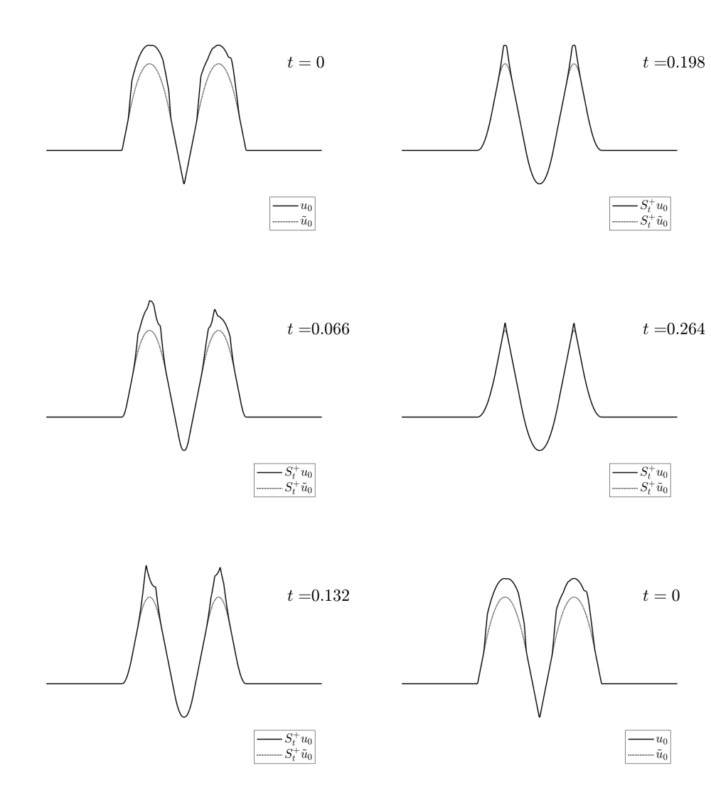
In this case, due to the presence of the nonlinear term H(\nabla_x u) in the equation, one cannot in general expect the existence of a regular C^1 solution, even if the initial condition u_0 is assumed to be very smooth. As we shall see, this loss of regularity results in a loss of information of the initial condition and the impossibility of uniquely determining u_0 from the observed solution at time T.
Our goal is, for a given observation u_T\in C^{0,1}(\mathbb{R}^n), determine all the initial conditions u_0 for which the solution u to (1) satisfies u(T,\cdot)= u_T, or equivalently, S_T^+u_0 =u_T.
We split the problem in three steps:
Step 1: We first determine if the observation u_T is admissible, i.e. if there exists at least one u_0 satisfying S_T^+ u_0=u_T.
The natural candidate is the one obtained by reversing the time in the equation (1), considering u_T as terminal condition.
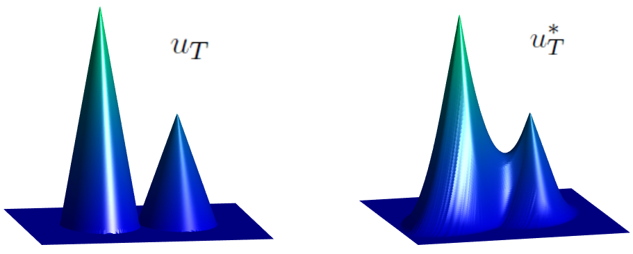
We denote by S_T^-u_T the backward in time solution at time t=0. In fact, it is proved in [1] that u_T is admissible if and only if the initial condition \tilde{u}_0 = S_T^- u_T satisfies S_T^+ \tilde{u}_T =u_T.
Step 2: Secondly, if the observation u_T is not admissible (it might be a consequence of noise effects or errors in the measurements) we compute the following projection of u_T on the set of admissible observations:
u_T^\ast : = S_T^+(S_T^- u_T).
Observe that, for any u_T, the projection u_T^\ast is, by definition, admissible. In [1], it is proven that, under suitable hypotheses on H, the function u_T^\ast is the unique viscosity solution to the nonlinear obstacle problem.
\min \left\{ v - u_T, \ -\lambda_n \left[ D^2 v - \dfrac{[H_{pp}(D v)]^{-1}}{T}\right] \right\} = 0.Here, for a symmetric n\times n matrix, \lambda_n[X] represents its greatest eigenvalue. The projection u_T^\ast is, in fact, the smallest admissible observation bounded from below by u_T.
Step 3: Finally, given an admissible observation u_T, or its projection if it were not admissible, we construct all the initial conditions u_0 satisfying S_T^+ u_0=u_T.
This construction is done in [1], and needs of only two ingredients:
(1) The backward solution \tilde{u}_0 = S_T^- u_T, obtained by reversing the time in (1);
(2) and the following subset of \mathbb{R}^n:
X_T(u_T) : = \left\{ z- T\, H_p (\nabla u_T(z)); \ \forall z\in\mathbb{R}^n \ \text{such that} \ u_T(\cdot) \ \text{is differentiable at} \ z\right\},obtained from the differentiability points of u_T.
Once these two elements are obtained, one can characterize the initial conditions u_0 satisfying S_T^+ u_0 =u_T as the functions that are bounded from below by \tilde{u}_0 in all \mathbb{R}^n and are equal to \tilde{u}_0 in X_T(u_T).
If, for an admissible observation u_T, we denote
I_T(u_T):= \left\{ u_0 \in C^{0,1}(\mathbb{R}^n)\, ; \ S_T^+ u_0 = u_T\right\},we can characterize this set of initial conditions as follows:
I_T(u_T) = \left\{ \tilde{u}_0 + \varphi \, ; \, \varphi\in C^{0,1}(\mathbb{R}^n)\ \text{such that} \ \varphi\geq 0\ \text{and}\ \text{supp} (\varphi) \subset \mathbb{R}^n\setminus X_T(u_T)\right\}.
Inverse Design for Hamilton-Jacobi Equation
We point out that, given an admissible observation u_T, the initial state u_0 can be uniquely determined if and only if X_T(u_T)=\mathbb{R}^n.
This is the case when the solution is C^1 in [0,T], however, as soon as the solution fails to be C^1 in [0,T], the set X_T(u_T) is a proper subset of \mathbb{R}^n and then the initial condition can no longer be uniquely determined in the region \mathbb{R}^n\setminus X_T(u_T) (white region in the right-hand-side plot).
References
[1] C. Esteve, E. Zuazua, The inverse problem for Hamilton-Jacobi equations and semiconcave envelopes, 2020 preprint arXiv:2003.06914
|| Go to the Math & Research main page


