Low-rank balanced truncation of bilinear systems via Laguerre functions

Low-rank balanced truncation of bilinear systems via Laguerre functions

 

1 Introduction

Bilinear systems are an important class of nonlinear systems which typically arise from approximating more involved nonlinearities by using the Carleman linearization approach or by imposing certain boundary conditions to discretized partial differential equations (PDEs). They can be considered as a bridge between linear and nonlinear systems. {Bilinear systems arise as natural models for biological processes and physical systems such as nuclear fission and heat transfer, and DC brush motors. In addition, they can be used to approximate large-scale nonlinear systems of the form

\left \{ \begin{aligned} & \dot{x}(t)=\textbf{f}(x(t),t)+\textbf{g}(x(t),t)u(t), \\ & y(t)=Cx(t), \end{aligned}\right. (1.1)

where \textbf{f} and \textbf{g} are analytic functions of the state, and continuous in t. Using the Carleman linearization, the nonlinear system \eqref{1.00} can be approximated by a bilinear system of the following form

\left \{ \begin{aligned} & \dot{x}(t)=Ax(t)+\sum_{i=1}^{m}N_ix(t)u_i(t)+Bu(t), \\ & y(t)=Cx(t), \end{aligned}\right. (1.2)

that matches a few terms in the Taylor series expansion of \textbf{f} and \textbf{g} around some equilibrium state. In this context, bilinear systems have been applied to the modeling of nonlinear RC circuits, microelectromechanical systems (MEMS) such as parallel plate electrostatic actuators, nonlinear heat transfer and stochastic control (a semidiscretized Fokker-Planck equation with external forcing).

The goal of Petrov-Galerkin projection model order reduction methods is to construct projection matrices V, W \in \mathbb{R}^{n\times r} (r\ll n) satisfying W^\mathrm{T}V=I, and generate a reduced model

\left \{ \begin{aligned} & \dot{\tilde{x}}(t)=\tilde{A}\tilde{x}(t)+\sum_{i=1}^{m}\tilde{N}_i\tilde{x}(t)u_i(t)+\tilde{B}u(t), \\ & \tilde{y}(t)=\tilde{C}^{\mathrm{T}}\tilde{x}(t), \end{aligned}\right. (1.3)

with initial condition \tilde{x}(0)=\tilde{x}_0, where
\tilde{x}_0=W^{\mathrm{T}}x_0, \tilde{A}=W^{\mathrm{T}}AV, \tilde{B}=W^{\mathrm{T}}B, \tilde{C}=V^{\mathrm{T}}C, and
\tilde{N}_i=W^{\mathrm{T}}N_iV, for i=1, 2, \ldots, m, such that the system should preserve as much properties of the original system as possible.

2 Balanced truncation of bilinear systems via low-rank Gramian approximation

The controllability (\mathcal{P}) and observability (\mathcal{Q}) Gramians of bilinear system (1.2) are defined as

\mathcal{P} = \sum_{i=1}^{\infty}\int_{0}^{\infty}\cdots\int_{0}^{\infty}\bar{P}_{i}\bar{P}_{i}^{\mathrm{T}}dt_{1}\cdots dt_{i}, (2.1)

\mathcal{Q} = \sum_{i=1}^{\infty}\int_{0}^{\infty}\cdots\int_{0}^{\infty}\bar{Q}_{i}\bar{Q}_{i}^{\mathrm{T}}dt_{1}\cdots dt_{i}, (2.2)

where

\begin{aligned} & \bar{P}_{1} = P_{1}(t_{1}) = e^{At_{1}}B, \quad \bar{Q}_{1} = Q_{1}(t_{1}) = e^{A^{\mathrm{T}}t_{1}}C^{\mathrm{T}},\\ & \bar{P}_{i} = P_{i}(t_{1}, \ldots, t_{i}) = \left[\begin{array}{cccc} e^{At_{i}}N_{1}\bar{P}_{i-1} & e^{At_{i}}N_{2}\bar{P}_{i-1} & \ldots & e^{At_{i}}N_{m}\bar{P}_{i-1} \end{array}\right], \\ & \bar{Q}_{i} = Q_{i}(t_{1}, \ldots, t_{i}) = \left[\begin{array}{cccc} e^{A^{\mathrm{T}}t_{i}}N_{1}^{\mathrm{T}}\bar{Q}_{i-1} & e^{A^{\mathrm{T}}t_{i}}N_{2}^{\mathrm{T}}\bar{Q}_{i-1} & \ldots & e^{A^{\mathrm{T}}t_{i}}N_{m}^{\mathrm{T}}\bar{Q}_{i-1} \end{array}\right], \quad i = 2, 3, \ldots \end{aligned}

These Gramians satisfy the following generalized algebraic Lyapunov equations:

A \mathcal{P} + \mathcal{P} A^{\mathrm{T}} + \sum_{i=1}^{m} N_{i} \mathcal{P} N_{i}^{\mathrm{T}} + B B^{\mathrm{T}} = 0,

A^{\mathrm{T}} \mathcal{Q} + \mathcal{Q} A + \sum_{i=1}^{m} N_{i}^{\mathrm{T}} \mathcal{Q} N_{i} + C^{\mathrm{T}} C = 0.

The connections between these Gramians and the energy functionals of bilinear systems have been studied in [3]. Furthermore, the relations between the Gramians and the controllability/observability of bilinear systems have also been studied therein. However, the main bottleneck in using these Gramians in the MOR context is the computation of the Gramians, though recently there have been many advances in methods to determine the low-rank solutions of these generalized Lyapunov equations. Here, we present a approximate low-rank decomposition of the Gramians \mathcal{P}, \mathcal{Q} of the bilinear system (1.2) based on the Laguerre functions.

2.1 Laguerre approximation of the matrix exponential function
For Re(a) \lt 0, we have the Laguerre expansion [4]

e^{at} = \sum_{k=0}^{\infty} a_{k} \phi_{k}^{\alpha}(t) \quad t \geq 0,

with the coefficients \{a_{k}\}_{k=0}^{\infty} defined by

\begin{aligned} a_{k} & = \int_{0}^{\infty} e^{at} \phi_{k}^{\alpha}(t) dt = \frac{\sqrt{2\alpha}}{\alpha-a}\Big(\frac{a+\alpha}{a-\alpha}\Big)^{k} \\ & = (-1)^{k} \sqrt{2\alpha} \big(a + \alpha\big)^{k} \big(\alpha - a\big)^{-(k+1)}. \end{aligned}

We now extend the above Laguerre expansion from e^{at} with Re(a) \lt 0 to the matrix exponential function e^{At} with stable A (A \in \mathbb{C}^{n \times n} is called stable if all its eigenvalues are strictly in the left-half of the complex plane). Then, it has

e^{At} = \sum_{k=0}^{\infty} A_{k} \phi_{k}^{\alpha}(t),
with the coefficient matrices \{A_{k}\}_{k=0}^{\infty} satisfying

A_{k} = (-1)^{k} \sqrt{2\alpha} \big( \alpha I + A \big)^{k} \big(\alpha I - A \big)^{-(k+1)},

where I is the identity matrix with appropriate dimension.

2.2 Low-rank decomposition of the Gramians \mathcal{P}, \mathcal{Q} based on Laguerre functions
First, we expand the matrix exponential function e^{At}B by a finite term Laguerre functions as the following approximate form:

e^{At}B \approx \sum_{i=0}^{N-1} A_{i}B\phi_{i}^{\alpha}(t),

where A_{i} = (-1)^{i} \sqrt{2\alpha} \big( \alpha I + A \big)^{i} \big(\alpha I - A \big)^{-(i+1)} \in \mathbb{R}^{n\times n}\ (i = 0, 1, \ldots, N-1) are the Laguerre coefficient matrices. Then, it has

\begin{aligned} \mathcal{P}_{1} & = \int_{0}^{\infty} \bar{P}_{1} \bar{P}_{1}^{\mathrm{T}} dt_{1} = \int_{0}^{\infty} e^{At} B B^{\mathrm{T}} e^{A^{\mathrm{T}}t} dt = \int_{0}^{\infty} (e^{At} B) (e^{At} B)^{\mathrm{T}} dt \\ & \approx \int_{0}^{\infty} \Big(\sum_{i=0}^{N-1} A_{i}B\phi_{i}^{\alpha}(t)\Big) \Big(\sum_{i=0}^{N-1} {A_{i}B\phi_{i}^{\alpha}(t)}\Big)^{\mathrm{T}} dt \\ & = \int_{0}^{\infty} \left[ \begin{array}{cccc} A_{0}B & A_{1}B & \cdots & A_{N-1}B \\ \end{array} \right] \left[ \begin{array}{c} \phi_{0}^{\alpha}(t) \\ \phi_{1}^{\alpha}(t) \\ \vdots \\ \phi_{N-1}^{\alpha}(t) \\ \end{array} \right] \\ & ~~~~~~ \cdot \left[ \begin{array}{cccc} \phi_{0}^{\alpha}(t) & \phi_{1}^{\alpha}(t) & \cdots & \phi_{N-1}^{\alpha}(t) \\ \end{array} \right] \left[ \begin{array}{c} (A_{0}B)^{\mathrm{T}} \\ (A_{1}B)^{\mathrm{T}} \\ \vdots \\ (A_{N-1}B)^{\mathrm{T}} \\ \end{array} \right] dt \\ & \approx \mathcal{F}_{1} \mathcal{F}_{1}^{\mathrm{T}}, \end{aligned}

where \mathcal{F}_{1} = \left[ \begin{array}{cccc} F_{1,0} & F_{1,1} & \ldots & F_{1,N-1} \\ \end{array} \right] \in \mathbb{R}^{n \times Nm} and

\begin{aligned} & F_{1,0} = \sqrt{2\alpha} (\alpha I - A)^{-1} B, \\ & F_{1,j} = \big[(A + \alpha I)(A - \alpha I)^{-1}\big] F_{1,j-1}, \quad j = 1, 2, \ldots, N-1. \end{aligned}

Consider the first two terms in the series in (2.1), which are dependent on the first two kernels of the Volterra series of the bilinear system

\begin{aligned} \mathcal{P}_{2} & = \int_{0}^{\infty} \bar{P}_{1} \bar{P}_{1}^{\mathrm{T}} dt_{1} + \int_{0}^{\infty} \int_{0}^{\infty} \bar{P}_{2} \bar{P}_{2}^{\mathrm{T}} dt_{1} dt_{2} \\ & = \int_{0}^{\infty} \bar{P}_{1} \bar{P}_{1}^{\mathrm{T}} dt_{1} + \int_{0}^{\infty} \int_{0}^{\infty} e^{At_{2}}\left[ \begin{array}{cccc} N_{1}\bar{P}_{1} & N_{2}\bar{P}_{1} & \ldots & N_{m}\bar{P}_{1} \\ \end{array} \right] \left[ \begin{array}{c} (N_{1}\bar{P}_{1})^{\mathrm{T}} \\ (N_{2}\bar{P}_{1})^{\mathrm{T}} \\ \vdots \\ (N_{m}\bar{P}_{1})^{\mathrm{T}} \\ \end{array} \right] e^{A^{\mathrm{T}}t_{2}} dt_{1} dt_{2} \\ & \approx \mathcal{F}_{1} \mathcal{F}_{1}^{\mathrm{T}} + \mathcal{F}_{2} \mathcal{F}_{2}^{\mathrm{T}}, \end{aligned}

where

\mathcal{F}_{2} = \left[ \begin{array}{cccc} F_{2,0} & F_{2,1} & \ldots & F_{2,N-1} \\ \end{array} \right] \in \mathbb{R}^{n \times N^{2}m^{2}}

and

\begin{aligned} & F_{2,0} = \sqrt{2\alpha} (\alpha I - A)^{-1} \left[ \begin{array}{cccc} N_{1}\mathcal{F}_{1} & N_{2}\mathcal{F}_{1} & \ldots & N_{m}\mathcal{F}_{1} \\ \end{array} \right], \\ & F_{2,j} = \big[(A + \alpha I)(A - \alpha I)^{-1}\big] F_{2,j-1},\quad j = 1, 2, \ldots, N-1. \end{aligned}

Then, for the truncated Gramian with the first l terms \mathcal{P}_{l} of the bilinear system, we have the following low-rank decomposition:

\mathcal{P}_{l} = \sum_{i=1}^{l}\int_{0}^{\infty}\cdots\int_{0}^{\infty}\bar{P}_{i}\bar{P}_{i}^{\mathrm{T}}dt_{1}\cdots dt_{i} \approx \mathcal{F} \mathcal{F}^{T}, (2.3)

where \mathcal{F} = \left[ \begin{array}{cccc} \mathcal{F}_{1} & \mathcal{F}_{2} & \ldots & \mathcal{F}_{l} \\ \end{array} \right] , \mathcal{F}_{i} = \left[ \begin{array}{cccc} F_{i,0} & F_{i,1} & \ldots & F_{i,N-1} \\ \end{array} \right] and

\left\{\begin{aligned} & F_{1,0} = \sqrt{2\alpha} (\alpha I - A)^{-1} B, \\ & F_{1,j} = \big[(A + \alpha I)(A - \alpha I)^{-1}\big] F_{1,j-1}, \quad j = 1, 2, \ldots, N-1 \\ & F_{i,0} = \sqrt{2\alpha} (\alpha I - A)^{-1} \left[ \begin{array}{cccc} N_{1}\mathcal{F}_{i-1} & N_{2}\mathcal{F}_{i-1} & \ldots & N_{m}\mathcal{F}_{i-1} \\ \end{array} \right], \\ & F_{i,j} = \big[(A + \alpha I)(A - \alpha I)^{-1}\big] F_{i,j-1}, \quad i = 2, 3, \ldots, l. \end{aligned} \right.

Similarity to the decomposition of \mathcal{P}_{l}, the truncated observability Gramian with the first l terms \mathcal{Q}_{l} of the bilinear system has the following low-rank approximation form:

\mathcal{Q}_{l} = \sum_{i=1}^{l}\int_{0}^{\infty}\cdots\int_{0}^{\infty}\bar{Q}_{i}\bar{Q}_{i}^{\mathrm{T}}dt_{1}\cdots dt_{i} \approx \mathcal{G} \mathcal{G}^{T}, (2.4)

where \mathcal{G} = \left[ \begin{array}{cccc} \mathcal{G}_{1} & \mathcal{G}_{2} & \ldots & \mathcal{G}_{l} \\ \end{array} \right] , \mathcal{G}_{i} = \left[ \begin{array}{cccc} G_{i,0} & G_{i,1} & \ldots & G_{i,N-1} \\ \end{array} \right] and

\left\{\begin{aligned} & G_{1,0} = \sqrt{2\alpha} (\alpha I - A^{\mathrm{T}})^{-1} C^{\mathrm{T}}, \\ & G_{1,j} = \big[(A^{\mathrm{T}} + \alpha I)(A^{\mathrm{T}} - \alpha I)^{-1}\big] G_{1,j-1}, \quad j = 1, 2, \ldots, N-1 \\ & G_{i,0} = \sqrt{2\alpha} (\alpha I - A^{\mathrm{T}})^{-1} \left[ \begin{array}{cccc} N_{1}^{\mathrm{T}}\mathcal{G}_{i-1} & N_{2}^{\mathrm{T}}\mathcal{G}_{i-1} & \ldots & N_{m}^{\mathrm{T}}\mathcal{G}_{i-1} \\ \end{array} \right], \\ & G_{i,j} = \big[(A^{\mathrm{T}} + \alpha I)(A^{\mathrm{T}} - \alpha I)^{-1}\big] G_{i,j-1}, \quad i = 2, 3, \ldots, l. \end{aligned} \right.

2.3 Basic algorithm
According to the low-rank factors \mathcal{F} and \mathcal{G}, we can use the low-rank square root method (LRSRM) [5] to generate the ROM. The reduction procedure can be described by Algorithm 1. {Algorithm 1 is a Petrov-Galerkin projection (S_{r} \neq T_{r}). The main disadvantage is that it may lead to numerical errors and instabilities. To alleviate such shortcoming, we use a modification of the dominant subspaces projection model reduction (DSPMR) [5] to modify the above algorithm. The idea behind DSPMR is, instead of balancing controllability and observability Gramians, to combine the associated principal subspaces obtained from approximate system Gramians. This yields a simple algorithm which is based upon low-rank factors of the controllability and observability Gramians. The modified algorithms are given by Algorithm 2 and Algorithm 3 as follows.}
Algorithm 1: Laguerre-Gramian-based LRSRM for bilinear systems (LG-LRSRM(BL))}
Input: A, B, C, N_{i}, N, l, \alpha, tol: tolerance for the approximation error of the ROM;
Output: ROM of order r: \tilde{A}, \tilde{N}_{i}, \tilde{B}, \tilde{C};
1. Compute the low-rank factors \mathcal{F} and \mathcal{G} from (2.3) and (2.4);
2. Compute the SVD: \mathcal{G}^{\mathrm{T}} \mathcal{F} = \mathcal{U} {\Sigma} \mathcal{V}^{\mathrm{T}}, \mathcal{U}_{r} = \mathcal{U}(:,1:r), \mathcal{V}_{r} = \mathcal{V}(:,1:r), and {{{\Sigma}_{r} = {\Sigma}(1:r,1:r)}}; r is adaptively chosen by given tolerance: \delta = 2 \sum_{j=r+1}^{r_{N}} \tilde{\sigma}_{j} \leq <em>tol</em>; 3. Compute projection matrices: \mathcal{T}_{r} = \mathcal{F} \mathcal{V}_{r} {\Sigma}_{r}^{-\frac{1}{2}}, \quad \mathcal{S}_{r} = \Sigma_{r}^{-\frac{1}{2}} {\mathcal{U}_{r}}^{\mathrm{T}} \mathcal{G}^{\mathrm{T}};
4. Construct the ROM: \tilde{A} = \mathcal{S}_{r} A \mathcal{T}_{r}, \tilde{N}_{i} = \mathcal{S}_{r} N_{i} \mathcal{T}_{r}, \tilde{B} = \mathcal{S}_{r} B, \tilde{C} = C \mathcal{T}_{r}.

Algorithm 2: Laguerre-Gramian-based DSPMR for bilinear systems (LG-DSPMR(BL))
Input: A, B, C, N_{i}, N, \alpha, r;
Output: \tilde{A}, \tilde{B}, \tilde{C}, \tilde{N}_{i};
1. Compute low-rank factors \mathcal{F} and \mathcal{G} from (2.3) and (2.4);
2. Compute the SVDs: \mathcal{F} = \mathcal{U}_{F} \Sigma_{F} \mathcal{V}_{F}^{\mathrm{T}}, \mathcal{G} = \mathcal{U}_{G} \Sigma_{G} \mathcal{V}_{G}^{\mathrm{T}};
3. Choose \tilde{r}/{2} \leq k \leq \verb"min"\{ r_{\mathcal{F}}, r_{\mathcal{G}} \}, \tilde{r} is adaptively chosen by given tolerance: {\delta = 2 \sum_{j={r}+1}^{r_{N}} \tilde{\sigma}_{j} \leq <em>tol</em>;} 4. Compute the QR decomposition: \big[\mathcal{U}_{F}(:,1:k), \quad \mathcal{U}_{G}(:,1:k)\big] = Q R, \mathcal{V} = Q(:,1:r);
5. Construct the ROM: \tilde{A} = \mathcal{V}^{\mathrm{T}} A \mathcal{V}, \tilde{N}_{i} = \mathcal{V} N_{i} \mathcal{V}, \tilde{B} = \mathcal{V}^{\mathrm{T}} B, \tilde{C} = C \mathcal{V}.

Algorithm 3: Laguerre-Gramian-based refined DSPMR for bilinear systems (LG-RDSPMR(BL))
Input: A, B, C, N_{i}, N, \alpha, r;
Output: \tilde{A}, \tilde{B}, \tilde{C}, \tilde{N}_{i};
1. Compute low-rank factors \mathcal{F} and \mathcal{G} from (2.3) and (2.4);
2. Compute the SVD: \Big[ \frac{1}{\| \mathcal{F} \|_{F}}\mathcal{F} \quad \frac{1}{\| \mathcal{G} \|_{F}}\mathcal{G} \Big] = \mathcal{U} \Sigma \mathcal{V}^{\mathrm{T}}, \mathcal{S} = \mathcal{U}(:,1:r);
3. Construct the ROM: \tilde{A} = \mathcal{S}^{\mathrm{T}} A \mathcal{S}, \tilde{N}_{i} = \mathcal{S}^{\mathrm{T}} N_{i} \mathcal{S}, \tilde{B} = \mathcal{S}^{\mathrm{T}} B, \tilde{C} = C \mathcal{S}.

3 Numerical example: Nonlinear Heat Transfer Model

In this example, a bilinear model for a nonlinear heat transfer problem is constructed. The physical system to be modeled in Figure \ref{figbeam} is the heat transfer along a 1D beam with length L, cross sectional area S, and nonlinear heat conductivity represented by a polynomial in temperature T(x, t) of arbitrary degree N

\kappa(T) = a_{0} + a_{1} T +\cdots + a_{N} T^{N}. (3.1)

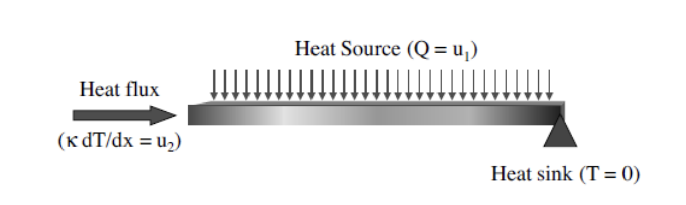
Figure 1. The modeled beam with heat flux inputs and heat sink.

The right end of the beam (at x = L) is fixed at ambient temperature. The model has two inputs: a time-dependent uniform heat flux u_1(t) at the left end (at x = 0) and a time-dependent heat source u_2(t) distributed along the beam. Including the nonlinear heat conductivity in the differential form of the heat transfer equation gives

-\nabla \cdot (\kappa(T)\nabla T) + \rho c_{p} \dot{T} = u_{2}(t), (3.2)

where \rho is the material density, and c_p is the heat capacity. Applying the definition of \kappa(T) to this equation yields the heat transfer system governed by the equations

-\sum_{i=0}^{N}a_{i} \nabla \cdot (T^{i} \nabla T) + \rho c_{p} \dot{T} = u_{2}(t). (3.3)

Applying the Carleman linearization, we derive the following bilinear realization for a quadratic approximation:

A = \left[ \begin{array}{cc} A_1 & A_2 \\ 0 & A_1 \otimes I_{n} + I_{n} \otimes A_1 \\ \end{array} \right], \quad N_{k} = \left[ \begin{array}{cc} 0 & 0 \\ B_{k} \otimes I_{n} + I_{n} \otimes B_{k} & 0 \\ \end{array} \right]\quad \text{for}\quad k = 1, 2, \mathcal{B} = \left[ \begin{array}{c} E^{-1}B \\ 0 \\ \end{array} \right], \quad C.

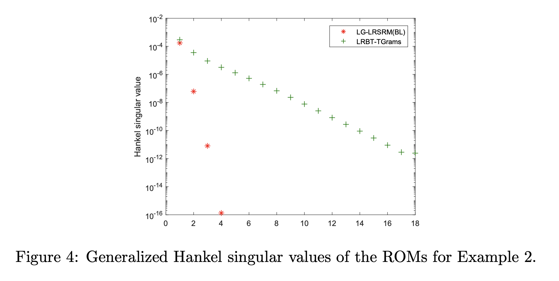
In our numerical simulation, the number of nodes of the original nonlinear system is 100, yielding a bilinear system of dimension 10100 with 2 inputs and 1 output, taken as the first or the middle node in the discretization. The computational times for constructing and simulating ROMs by different methods and maximum relative errors are reported in Table 1. Figure 2(a) and Figure 3(a) show the steady state temperatures of the original nonlinear heat transfer model at the leftmost and the middle of the beam for an input of 5 \cdot 10^{4} W/m^{2}, and the corresponding relative errors of these ROMs are shown in Figure 2(b) and Figure 3(b). For comparison between the different MOR methods and evaluating their accuracy, all the models are simulated with the same input and measuring point. All values used in the simulation are relative to an ambient temperature of 300 K. Furthermore, the approximate generalized Hankel singular values (HSVs) of Algorithm 1 and LRBT-TGrams are plotted in Figure 4.

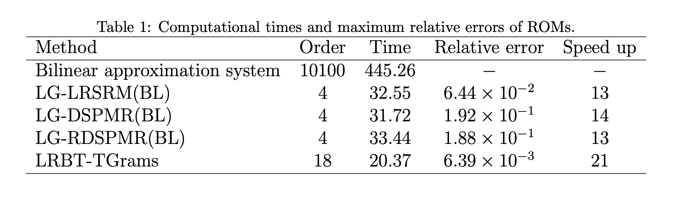
Table 1. Computational times and maximum relative errors of ROMs.

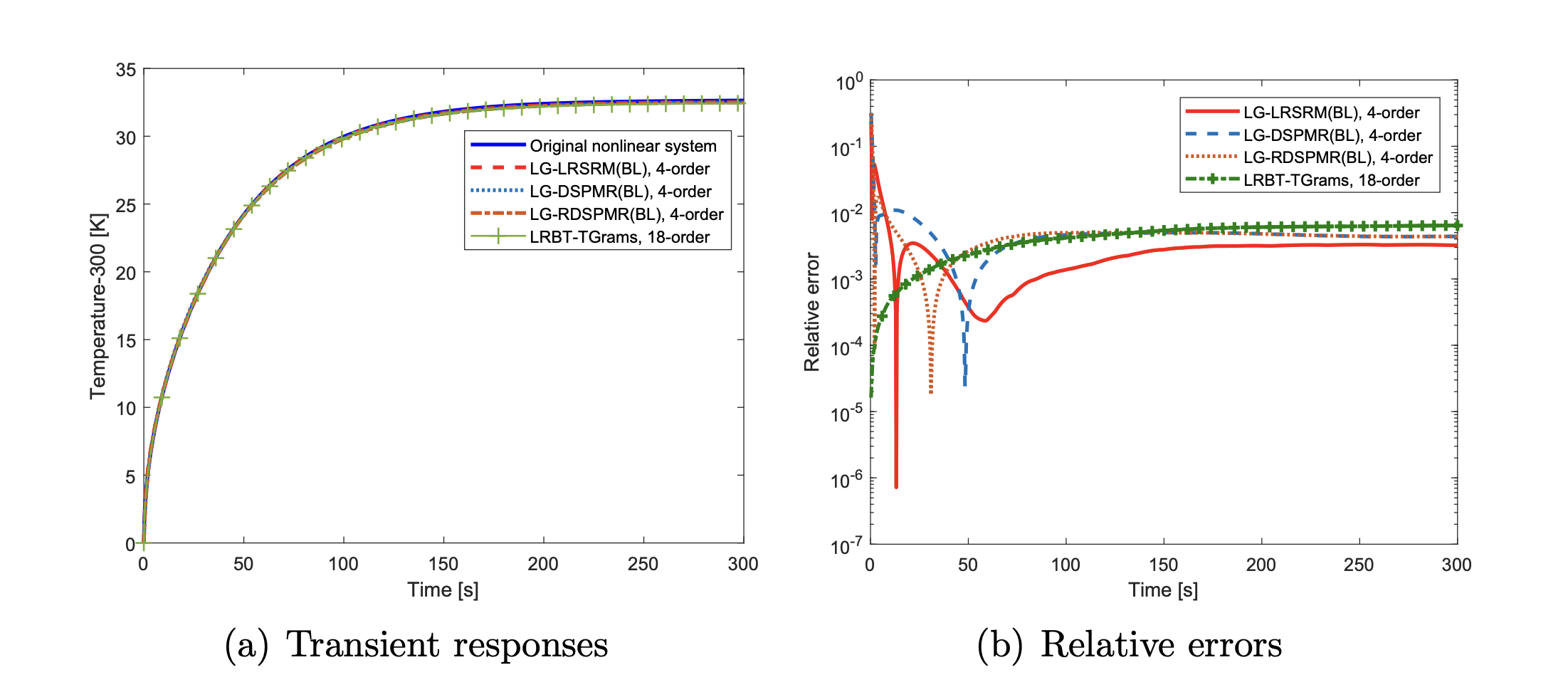
Figure 2. Transient responses of the nonlinear heat transfer model for the temperature at the leftmost end for an input of 5 \cdot 10^{4} W/m^{2}, and the relative errors \varepsilon of the ROMs with respect to the original system.

4 Conclusions

We mainly discuss the MOR for bilinear systems based on low-rank Gramian approximation. A series of MOR algorithms via Laguerre functions are presented. The proposed methods are much efficient in time, which is due to that the low-rank factors are constructed from a recurrence formula. At the same time, our modified algorithms with the ideas of DSPMR can produce stable ROMs under certain conditions. Carleman bilinearization is a systematical approach to perform quadratic approximation to a nonlinear system with nonlinear analytic functions. Although the dimension of the resulting bilinear system increases exponentially, the order of our acceptable ROMs is only 4\% of that of the original system when we take advantage of the underlying structure.

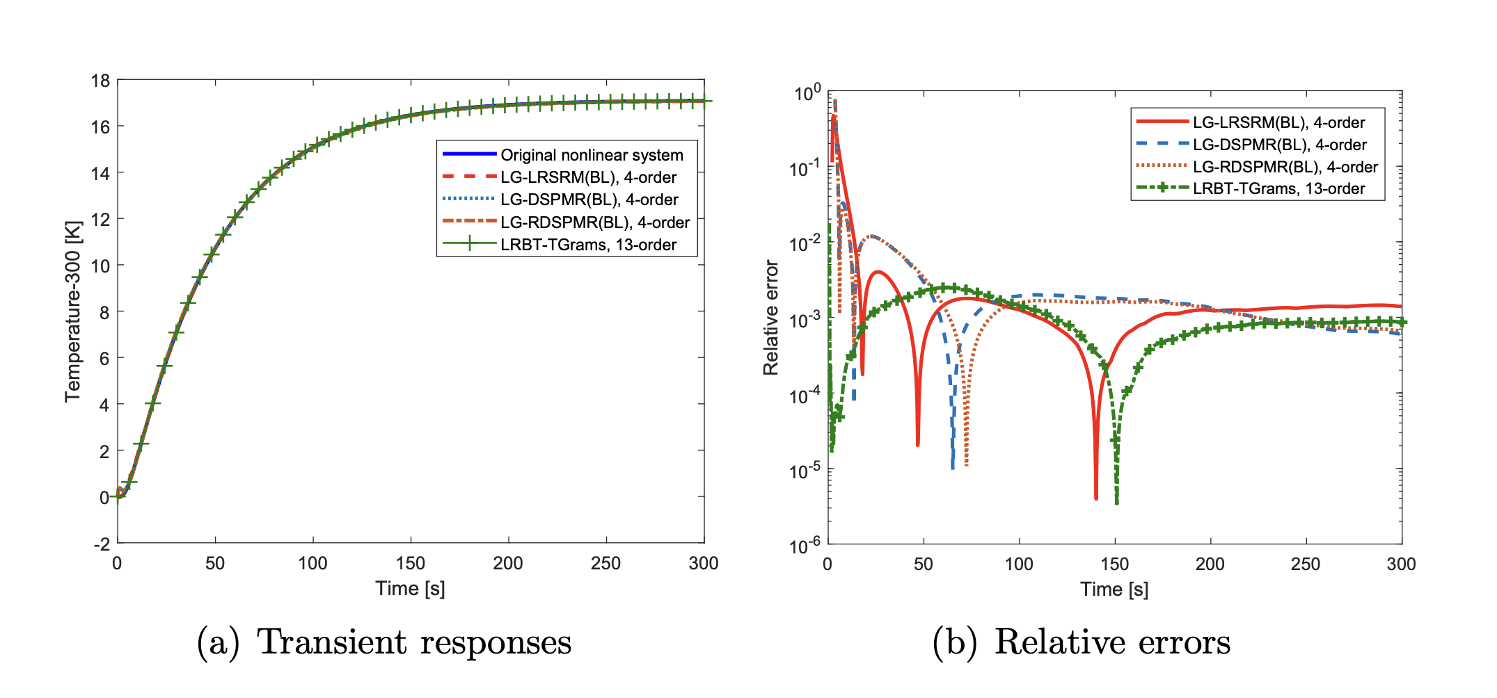
Figure 3. Transient responses of the nonlinear heat transfer model for the temperature at the leftmost end for an input of 5 \cdot 10^{4} W/m^{2}, and the relative errors \varepsilon of the ROMs with respect to the original system.

References

[1] Z.H. Xiao, Q.Y. Song, Y.L. Jiang, Z.Z. Qi, Model order reduction of linear and bilinear systems via low-rank Gramian approximation, Applied Mathematical Modelling 106 (2022) 100–113.
[2] Q.Y. Song, X. Du, Z.H. Xiao, Model order reduction based on low-rank decomposition of the cross Gramian, International Journal of Control (2023) 1–13.
[3] P. Benner, T. Damm, Lyapunov equations, energy functionals, and model order reduction of bilinear and stochastic systems, SIAM Journal on Control and Optimization 49 (2) (2011) 686–711.
[4] G. Moore, Orthogonal polynomial expansions for the matrix exponential, Linear Algebra and its Applications 435 (3) (2011) 537–559.
[5] T. Penzl, Algorithms for model reduction of large dynamical systems, Linear Algebra
and its Applications 415 (2-3) (2006) 322–343.

 

|| Go to the Math & Research main page

 

You might like!