Probabilistic Constrained Optimization on Flow Networks

This research was funded by DFG in the SFB Transregio 154: Mathematical modelling, simulation and optimization using the example of gas networks.

Uncertainty often plays an important role in the context of flow problems. We analyze a stationary and a dynamic flow model with uncertain boundary data and we consider optimization problems with probabilistic constraints in this context. The main difficulty is to evaluate probabilistic constraints of the form

$\mathbb{P} \left(\ b \in M\ \right) \geq \alpha,$

where $b$ is a realization of some random variable $\xi$ , $M$ is the set of feasible loads and $\alpha$ is a probability level. In this context feasible means, that the state corresponding to the random boundary data meets some box constraints. In general this probability can be computed by integrating the probability density function of the random variable $\xi$ over the feasible set $M$ but this can be difficult due to a high dimensional integral or an arbitrary, non convex and non smooth set $M$ .

Spheric Radial Decomposition (SRD) and Kernel Density Estimation (KDE)

For computing the probability, we use two different tools. The first one is the Spheric Radial Decomposition (SRD) which reduces the dimension of integration. For Gaussian distributed random variables with zero mean and correlation $R$ the SRD is defined as follows:

$\mathbb{P}\left(\ \zeta \in M\ \right) = \int_{\mathbb{S}^{n-1}} \mu_\chi \left\{\ r \geq 0\ \vert\ r L v \in M\ \right\}\ d\mu_{\eta} (v).$

The second tool is a Kernel Density Estimator (KDE), which allows us to estimate probability density functions with unknown probability distributions. For an independent and identically distributed sampling $\mathcal{Y} = \{y^1, \cdots, y^N\} \subseteq \mathbb{R}^n$ of a random variable $Y$ , a kernel function $K : \mathbb{R}^n \rightarrow \mathbb{R}$ and a bandwidth matrix $H \in \mathbb{R}^{n \times n}$ the KDE $\varrho_N : \mathbb{R}^n \rightarrow \mathbb{R}$ is defined as

$\varrho_N(z) = \frac{1}{N \det(H)^{\frac{1}{2}}} \sum_{i=1}^N K \left( H^{-\frac{1}{2}} (z - y^i) \right).$

Stationary States on Gas Networks
We consider a stationary model for the gas transport in a pipeline network including the Weymouth equation for the pressure loss along the pipes, conservation of mass and continuity of pressure at the network junctions, inlet pressure $p_0$ and random gas outflow $b$ . The feasible set is defined by box constraints for the pressure $p^{\min}, p^{\max}$ at the outflow nodes.

We use an explicit solution of the model to characterize the feasible set in terms of inequalities. This allows us compute the one dimensional sets

$\{\ r \geq 0\ \vert\ r L v \in M\ \},$

as union of disjoint intervals and thus we are able to apply the SRD to compute the probability for a random gas outflow to be feasible.

Further we define a sampling of the random gas outflow and use the KDE to estimate the probability density function of the pressures at the outflow nodes. For Gaussian product kernels and an appropriate choice for the bandwidth matrix the probability for a random gas outflow to be feasible can be computed by integrating the estimated probability density function of the pressures over the box constraints, which is

$\mathbb{P}(\ b \in M\ ) = \int_{p^{\min}}^{p^{\max}} \varrho_{p,N}(z)\ dz.$

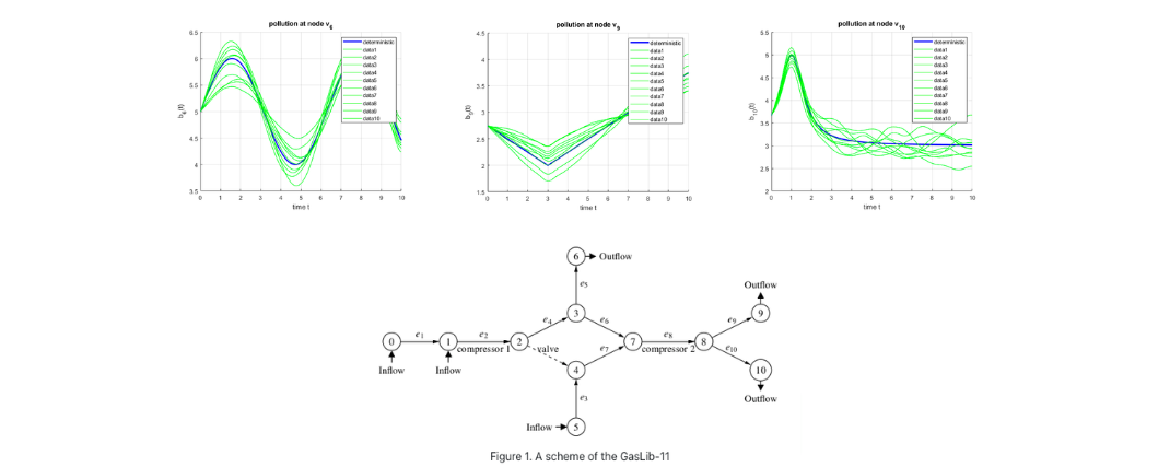
We consider a realistic gas network with $11$ node that is shown in Figure 1 and that can be found on GasLib. For

$p_0~=~ [60, 58, 60]^\top, \\ p^{\min}~=~[40, 40, 40]^\top, \\ b~=~[20, 15, 18]^\top,$

we compute the lowest upper pressure bound s.t. the pressures at the outflow nodes satisfy the box constraints, which is

$p^{\max}_{\text{det}} = \begin{bmatrix} 46.10 \\ 52.04 \\ 51.08 \end{bmatrix}.$

Then we assume that the gas outflow is random, $b \sim \mathcal{N}(\mu, \Sigma)$ with

$\mu = [20, 15, 18]^\top, \quad \Sigma = \begin{bmatrix} 2 & 0 & 0 \\ 0 & 2 & 0 \\ 0 & 0 & 2 \end{bmatrix}.$

With this we compute the lowest upper pressure bound, s.t. the pressures at the outflow nodes satisfy the box constraints in at least $75\%$ of all scenarios, which is

$p^{\max}_{\text{prob}} = \begin{bmatrix} 47.52 \\ 52.34 \\ 52.45 \end{bmatrix}.$

This slight increase in the upper pressure bound guarantees that in $75\%$ of all scenarios the pressure at the outflow nodes satisfies the probabilistic pressure bound $p^{\max}_{\text{prob}}$ , while the deterministic bound $p^{\max}_{\text{det}}$ is only satisfied in about $35\%$ of all scenarios.

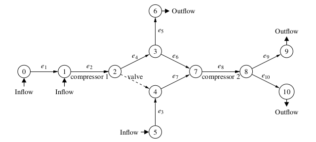
Figure 1. A scheme of the GasLib-11

Water Contamination Dynamics

Consider a water network equilibrium that is contaminated at some network junctions. The contamination $b(t)$ distributes through the pipes over time, which is modeled by a linear scalar transport equation. The contamination rate is uncertain over time, which is modeled by random Fourier series. The feasible set is defined by contamination bounds $r^{\min}, r^{\max}$ at the outflow nodes. The aim here is to evaluate the so-called probust (probabilistic and robust) constraint

$\mathbb{P}(\ b \in M(t) \quad \forall t \in [0, T]\ ) \geq \alpha,$

which means that $\alpha\%$ of all scenarios should always satisfy the contamination bounds.

We use the KDE approach for this setting as follows:
We define a sampling for the contamination scenarios and compute the (time dependent) contamination rate at the outflow nodes. The contamination bounds are satisfied if and only if the minimal and the maximal contamination rates satisfy the contamination bounds. So we use the KDE to estimate the probability density function of the minimal and maximal contamination rates $\varrho_{r,N}$ at the outflow nodes. So we can use the theory from the stationary case but the dimension doubles. Then the probability that a random contamination always satisfies the contamination bounds can be computed by

$\mathbb{P}(\ b \in M(t) \quad \forall t \in [0,T]\ ) = \int_{[r^{\min}, r^{\max}] \times [r^{\min}, r^{\max}]} \varrho_{r,N}(z)\ dz.$

We consider a realistic network with $11$ nodes that is shown in Figure 3. For

$b_6(t) = \sin(t) + 5, \\ b_9(t) = \frac{1}{4} \vert t - 3 \vert + 2, \\ b_{10}(t) = \frac{1}{(t-1)^2 + \frac{1}{2}} + 3, \\ r^{\min} = [3.5, 4, 1]^\top,$

we compute the lowest upper contamination bound s.t. the contamination rate at the outflow nodes always satisfy the bounds, which is

$r^{\max}_{\text{det}} = \begin{bmatrix} 5.78 \\ 6.39 \\ 2.51 \end{bmatrix}.$

We randomize the Fourier series of the boundary functions $b_6, b_9, b_{10}$ by Gaussian numbers with mean $1$ and \linebreak variance $0.1$ (see Figure 2).

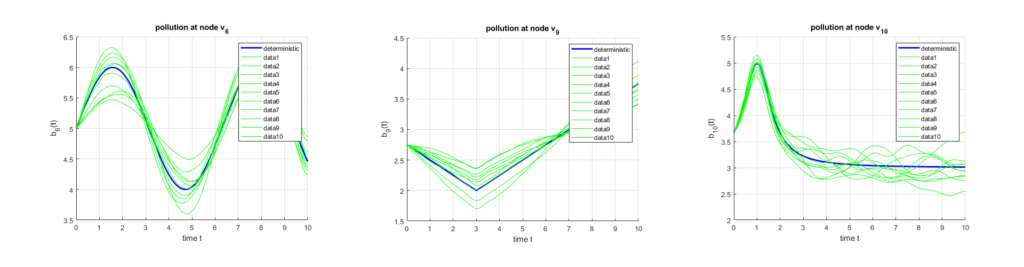
Figure 2: Random boundary scenarios at $v_6$ , $v_9$ and $v_{10}$

We compute the lowest upper contamination bound s.t. the contamination rate at the outflow nodes satisfies the contamination bounds at any time in at least 75% of all scenarios, which is
$r^{\max}_{\text{prob}} = \begin{bmatrix} 5.94 \\ 6.56 \\ 2.58 \end{bmatrix}.$

As in the stationary case this slight increase in the upper contamination bound guarantees that in $75\%$ of all scenarios the probabilistic contamination bound $r^{\max}_{\text{prob}}$ is satisfied at any time, while the deterministic bound $r^{\max}_{\text{det}}$ is only satisfied in about $38\%$ of all scenarios.

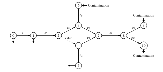
Figure 3: A network scheme for water pollution

References

[1] M. Schuster, E. Strauch, M. Gugat, J. Lang, Probabilistic Constrained Optimization on Flow Networks, Optim. Eng. (2021), https://doi.org/10.1007/s11081-021-09619-x