
Randomized time-splitting in linear-quadratic optimal control
Daniël Veldman, FAU DCN-AvH
Introduction
Solving an optimal control problem for a large-scale dynamical system can be computationally demanding. This problem appears in numerous applications. One example is Model Predictive Control (MPC), which requires the solution of several optimal control problems on a receding time horizon [5, 7]. Another example is the training of Deep Neural Networks (DNNs), which can be approached as an optimal control problem for a large-scale nonlinear dynamical system, see, e.g., [3, 1, 4, 8]. Because the computational cost for gradient based deterministic optimization algorithms explodes on large training data sets, Neural Networks (NNs) are typically trained using stochastic optimization algorithms such as stochastic gradient descent or stochastic (mini-)batch methods, see, e.g., [2]. In such methods, the update direction for the parameters of the NN is not computed based on the complete training data set, but on a subset of the available training data that is chosen randomly in each iteration. It can be shown that such methods converge in expectation to a (local) minimum of the considered cost functional, see, e.g., [2].
These successes inspired the development of Random Batch Methods (RBMs) for the simulation of interacting particle systems [6]. Because the number of interactions between N particles is of order N^2, the forward simulation of a system with a large number of particles is computationally demanding. A RBM reduces the required computational cost by reducing the number of considered interactions to an order of PN, where P is the size of the randomly chosen batches, and a significant reduction in computational time can be achieved when P \ll N. It can be shown that the expected error introduced by this process is proportional to \sqrt{h}, where h denotes (an upper bound on) the length of the considered time intervals, see [6]. The computation of optimal controls for interacting particle systems is even more computationally demanding than the forward simulation because it requires several simulations of the forward dynamics and the associated adjoint (backward) problem. It was therefore proposed in [7] to use a randomized algorithm for the optimal control of interacting particle systems, but a rigorous proof of convergence of the proposed method was still missing.
In this post, we present such convergence results for the classical Linear-Quadratic (LQ) setting. Extensions of these results to a nonlinear setting are not only of interest for the control of interacting particle systems as considered in [7], but have also applications in the training of certain DNNs which can be viewed as (the time discretization) of an optimal control problem, see, e.g., [3, 1, 4, 8]. The results for the LQ problem presented here form a starting point for the study of these more involved problem settings.
Proposed method
We consider the classical (finite-dimensional) LQ optimal control problem in which we want to find the control u^∗(t) that minimizes
J(u) = \frac{1}{2}\int_0^T \left( (x(t)-x_d(t))^\top Q (x(t)-x_d(t))+u(t)^\top R u(t) \right) \ \mathrm{d}t,
(1)
subject to the dynamics
![]() x(0) = x_0.
x(0) = x_0.
(2)
To speed up the computation of the minimizer u^*(t) of the original problem (1)-(2), the matrix A is written as the sum of M submatrices A_m
A = \sum_{m=1}^M A_m.
(3)
Typically, the submatrices A_m will be more sparse than the original matrix A. For ease of presentation, the results in this post are presented under the following assumption.
Assumption 1. The submatrices A_m in (3) are dissipative, i.e. \langle x, A_m x \rangle ≤ 0 for all x ∈ R^N and all m ∈ {1, 2,.., M}.
We then choose a temporal grid in the time interval [0, T]
0 = t_0 < t_1 < t_2 < ... < t_{K-1} < t_K = T
(4)
and denote
h_k = t_k - t_{k-1}, h = \max_{k \in \{1,2,..., K\}} h_k.
(5)
In each of the K subintervals [t_{k-1}, t_k), we randomly select a subset of indices in {1,2,..., M}. The idea of the proposed method is to consider only the submatrices A_m with the indices that have been selected for each time interval. To make this idea more precise, we enumerate all of the 2^M subsets of {1, 2,..., M} as {S_1, S_2,...S_{2^M}}. Note that one of the subsets S_{\ell} will be the empty set. To every subset S_\ell (\ell \in \{1, 2,..., 2^M \}) we then assign a probability p_\ell with which this subset is selected. This probability is the same in each of the time intervals [t_{k-1},t_k). Because we select only one subset S_\ell in each time interval, the probabilities p_\ell should satisfy
\sum_{\ell = 1}^{2^M} p_\ell = 1.
(6)
From the chosen probabilities p_\ell, we then compute the probability \pi_m that an index m \in {1,2,..., M} is an element of the selected subset
\pi_m = \sum_{\ell \in \mathcal{L}_m} p_\ell, \qquad \qquad \mathcal{L}_m = \{ \ell \in \{1,2, \ldots, 2^M \} \mid m \in S_\ell \}.
(7)
We need the following (weak) assumption on the selected probabilities p_\ell.
Assumption 2. The probabilities p_\ell (\ell \in {1,2,...,2^M}) are assigned such that
- (6) is satisfied and
- the probabilities \pi_m defined in (7) are positive for all m \in {1, ,2,..., M}.
In each of the K time intervals [t_{k-1},t_k), we then randomly select an index \omega_k \in {1,2, \ldots , 2^M} according to the chosen probabilities p_\ell (and independently of the other indices \omega_1, \omega_2, ... \omega_{k-1}, \omega_{k+1}, \omega_{k+1},..., \omega_K). The selected indices form a vector
\omega := (\omega_1, \omega_2, \ldots , \omega_K) \in \{1,2,\ldots ,2^M \}^K =: \Omega.
(8)
For the selected \omega \in \Omega, we then define a piece-wise constant matrix t \mapsto \mathcal{A}_h(\omega,t)
\mathcal{A}_h(\omega, t) = \sum_{m \in S_{\omega_k}} \frac{A_m}{\pi_m}, \qquad \qquad t \in [t_{k-1}, t_k).
(9)
The scaling by 1/\pi_m assures that the expected value of \mathcal{A}_h is A because
\sum_{\ell=1}^{2^M} \sum_{m \in S_{\omega_k}} \frac{A_m}{\pi_m} p_\ell = \sum_{m=1}^M \sum_{\ell \in \mathcal{L}_m} \frac{A_m}{\pi_m} p_\ell = \sum_{m=1}^M \frac{A_m}{\pi_m}\pi_m = \sum_{m=1}^M A_m = A,
(10)
where the first identity follows after interchanging the two summations using the definition of \mathcal{L}_m in (7), the second from the definition of \pi_m in (7), and the last identity from the decomposition of A in (3).
Example 1. In the simplest situation, we decompose the original matrix A into M = 2 matrices as A = A_1 + A_2. We then need to assign 2^M = 4 probabilities p_\ell to the subsets S_1 = { 1 }, S_2 = { 2 }, S_3 = { 1,2 }, and S_4 = \emptyset. In this example, we choose p_1 = p_2 = \tfrac{1}{2} and p_3 = p_4 = 0. This choice indeed satisfies Assumption 2 because \pi_1 = p_1 + p_3 = \tfrac{1}{2} > 0 and \pi_2 = p_2 + p_3 = \tfrac{1}{2} > 0. The matrix \mathcal{A}_h(\omega,t) is thus either equal to 2A_1 with probability p_1 = \tfrac{1}{2} or equal to 2A_2 with probability p_2 = \tfrac{1}{2}. The expected value of \mathcal{A}_h is then indeed \tfrac{1}{2} 2 A_1 + \tfrac{1}{2} 2 A_2 = A_1 + A_2 = A.
To reduce the computational cost for solving (2), the matrix A is replaced by a \mathcal{A}_h(\omega,t) in the RBM. For the selected vector of indices \omega \in \Omega, we thus obtain a solution t \mapsto x_h(\omega,t)
![]() x_h(\omega,0) = x_0.
x_h(\omega,0) = x_0.
(11)
We then consider the minimization of the functional
J_h(\omega, u) = \frac{1}{2}\int_0^T \left( (x_h(\omega,t)-x_d(t))^\top Q (x_h(\omega,t)-x_d(t))+u(t)^\top R u(t) \right) \ \mathrm{d}t,
(12)
over all u \in L^2(0,T) subject to the dynamics (11). The minimizer of J_h(\omega, \cdot) depends on the selected indices \omega \in \Omega and is denoted by u^*_h(\omega,t).
We consider x_h(\omega,t) and u_h^*(\omega,t) as approximations of x(t) and u^*(t), respectively. The accuracy of this (randomly generated) approximation is characterized will be studied in the next section.
To conclude this section, the proposed approach to approximate the solution x(t) of (2) for a given control u(t) and/or the optimal control u^*(t) that minimizes J(\cdot) in (1) subject to (2) is summarized in Algorithm (1).
Algorithm 1: The proposed randomized time-splitting method
Step 1. Decompose the matrix A into M submatrices A_m as in (3), preferably such that Assumption 1 is satisfied.
Step 2. Enumerate the 2^M subsets of {1, 2,..., M} and assign probabilities p_1, p_2,..., p_{2^M} such that Assumption 2 is satisfied.
Step 3. Divide the considered time interval [0, T] into K subintervals [t_{k-1}, t_k) and choose an index \omega_k according to the selected probabilities in Step 2 for each subinterval. Store the selected indices in a vector \omega = (\omega_1, \omega_2, \ldots \omega_K).
Step 4. Compute the solution x_h(\omega,t) of the dynamics (11) for a certain given control u(t) and/or compute the control u^*(\omega,t) that minimizes J_h(\omega,\cdot) in (12) subject to the dynamics (11).
Main results
Clearly, the deviation of the randomized matrix \mathcal{A}_h(\omega,t) from the original matrix A will influence the accuracy of the obtained results. The deviation of \mathcal{A}_h(t) from A is measured by
\mathrm{Var}[\mathcal{A}_h] := \sum_{\ell=1}^{2^M} \big\Vert \sum_{m \in S_\ell} \frac{A_m}{\pi_m} - A \big\Vert ^2 p_\ell,
(13)
where \big\Vert \cdot \big\Vert denotes the operator norm.
Example 1 (continued). We again consider the situation from Example 1 in which A is decomposed into M=2 submatrices as A = A_1 + A_2 and \mathcal{A}_h(\omega,t) is either 2A_1 or 2A_2, both with probability \tfrac{1}{2}. We now compute the variance \mathrm{Var}[\mathcal{A}_h] according to (13) and find
\mathrm{Var}[\mathcal{A}_h] = \| 2A_1 - A \|^2 p_1 + \| 2A_2 - A \|^2 p_2 = \| A_1 - A_2 \|^2.
(14)
Our first main result is an estimate for the difference e_h(\omega,t) = x_h(\omega,t) - x(t) between the RBM-dynamics (11) and the original dynamics (2).
Main result 1. Assume that the input u(t) in (2) is the same as in the input u(t) in (11) and that Assumptions 1 and 2 hold, then
\mathbb{E}[|e_h(t)|^2] \leq C_{[A,B,x_0,T,u]} h \mathrm{Var}[\mathcal{A}_h],
(15)
for all t \in [0,T].
The expectation operator \mathbb{E} is taken w.r.t.\ all possible outcomes \omega \in \Omega. The constant C_{[A,B,x_0,T,u]} can be taken as (\| A\|T^2 + 2T)(|x_0|+|Bu|_{L^1})^2. The estimate thus only depends on the used submatrices A_m, the probabilities p_\ell, and the used temporal grid t_0,t_1,\ldots , t_K through h\mathrm{Var}[\mathcal{A}_h] defined in (13). The proof of Main result 1 is inspired by the proofs of convergence of the RBM in [6].
The estimate (15) shows that the expected squared error is proportional to the temporal grid spacing h. We can thus make the expected squared error in the forward dynamics arbitrary small by reducing the grid spacing. Note that Markov’s inequality shows that
\mathbb{P}[|e_h(\omega,t)| > \varepsilon] = \mathbb{P}[|e_h(\omega,t)|^2 > \varepsilon^2] < \cfrac{\mathbb{E}[|e_h(t)|^2]}{\varepsilon^2}.
(16)
The probability that we select an \omega \in \Omega for which |e_h(\omega,t)| exceeds any given treshold \varepsilon > 0 is thus controlled by \mathbb{E}[|e_h(t)|^2]. According to (15), we can make this probability as small as desired by choosing the temporal grid spacing h small enough. However, one should also keep in mind that decreasing h will increase the computational cost for the RBM-dynamics (11) and that the computational advantage of the RBM is lost when the required grid spacing is too small.
We now present the main results aimed at the LQ optimal control problem constrained by randomized dynamics. Because the optimal control u^*_h(\omega,t) depends on the selected indices \omega, we need the following result. The key difference with the first main result is that the input u_h(\omega,t) may now depend on the randomly selected indices \omega. This is a significant extension of Main result 1 because the dependence of the control on \omega makes the proof for the convergence of the RBM in [6] break down.
Note that replacing u(t) in (2) and (11) by u_h(\omega,t) results in solutions x(\omega,t) and x_h(\omega,t) that now both depend on the selected indices \omega. The second main result now gives a bound for the expected error e_h(\omega,t) = x_h(\omega,t) - x(\omega,t).
Main result 2. Consider any control u_h : \Omega \rightarrow L^2(0,T). Assume that Assumptions 1 and 2 are satisfied and let U be such that |u_h(\omega)|_{L^2(0,T)} \leq U for all \omega \in \Omega, then
\mathbb{E}[|e_h(t)|^2] \leq C_{[A,B,x_0,T,U]} h \mathrm{Var}[\mathcal{A}_h].
(17)
Just as in the first main result, the expectation is taken over all possible values of \omega \in \Omega and the constant C_{[A,B,x_0,T,U]} does not depend on the chosen submatrices A_m in (3), the chosen probabilities p_\ell, and the used temporal grid.
Using this result, we can now obtain a no-gap result which shows that the minimal value of the cost functional J_h(\omega, u_h^*(\omega)) is (in expectation) close to the minimal value J(u^*) in the original problem when h \mathrm{Var}[\mathcal{A}_h] is small enough.
Main result 3. Let u^*(t) be the control that minimizes the cost functional J(u) in (1) and let u_h^*(\omega,t) be the control that minimizes the cost functional J_h(\omega, u) in (12). Then
\mathbb{E}[|J_h(u^*_h) - J(u^*)|] \leq C_{[A,B,x_0,Q,R,x_d,T]} \left( \sqrt{h \mathrm{Var}[\mathcal{A}_h]} + h \mathrm{Var}[\mathcal{A}_h] \right).
(18)
The next main result shows that the optimal control for the RBM-problem u_h^*(\omega) also converges (in expectation) to the optimal control of the original problem u^* when h \rightarrow 0.
Main result 4. Let u_h^*(\omega,t) be the minimizer of J_h(\omega,\cdot) in (12) and u^*(t) be the minimizer of J in (1), then
\mathbb{E}[|u_h^* - u^*|_{L^2(0,T)}^2] \leq C_{[A,B,x_0,Q,R,x_d,T]} h \mathrm{Var}[\mathcal{A}_h].
(19)
The fourth main result justifies the use of the optimal control u^*_h(\omega), that is optimized for the RBM-dynamics, to the original dynamics, as proposed in [7].
When the control u^*_h(\omega) is close to the control u^* that is optimal for the original dynamics, the performance J(u^*_h(\omega)) should also be close to the optimal performance J(u^*). This idea is formalized by the fifth and last main result.
Main result 5. Let u^*(t) be the control that minimizes the cost functional J(u) in (1) and let u_h^*(\omega,t) be the control that minimizes the cost functional J_h(\omega, u) in (12). Then
\mathbb{E}[|J(u^*_h) - J(u^*)|] \leq C_{[A,B,x_0,Q,R,x_d,T]}h \mathrm{Var}[\mathcal{A}_h].
(20)
The fifth main result is particularly important because it shows that the performance J(u^*_h(\omega)) obtained with control u^*_h(\omega) optimized for the randomized dynamics is close to the optimal performance J(u^*) when h\mathrm{Var}[\mathcal{A}_h] is sufficiently small. This further motivates strategies in which the original system is controlled by controls u^*_h(\omega) that are optimized for the randomized dynamics, as was proposed in [7].
The proofs of the presented results are given in [9].
Numerical illustration
We consider a controlled heat equation on the a 1-D spatial domain [-L, L],
y_t(t,\xi) = y_{\xi\xi}(t,\xi) + \chi_{[-L/3,0]}(\xi) u(t), \xi \in [-L,L],
(21)
y_\xi(t,-L) = y_\xi(t,L) = 0, y(0,\xi) = e^{-\xi^2} + \xi^2e^{-L^2},
(22)
where \chi_{[-L/3,0]}(\xi) denotes the characteristic function for the interval [-L/3,0]. We want to compute the optimal controlu^*(t) that minimizes
\mathcal{J}(u) = \frac{100}{2}\int_0^T \int_{-L}^0 y(t,\xi)^2 \ \mathrm{d}\xi \ \mathrm{d}t + \frac{1}{2}\int_0^T u(t)^2 \ \mathrm{d}t.
(23)
We fix L = 1\tfrac{1}{2} and T = \tfrac{1}{2}.
The spatial discretization of the dynamics (21)-(22) is made by finite differences and the cost functional in (23) is discretized by the trapezoid rule. We choose a uniform spatial grid with N = 61 grid points \xi_i = (i-1)\Delta \xi - L (i \in \{ 1,2, \ldots , N \}), where \Delta \xi = 2L/(N-1) is the grid spacing. We thus obtain a problem of the form (1)-(2) in which the resulting A-matrix is
A = \frac{1}{\Delta \xi^2} \begin{bmatrix} -2 & 2 & 0 & \cdots & 0 & 0 & 0 \\ 1 & -2 & 1 & & 0 & 0 & 0 \\ 0 & 1 & -2 & & 0 & 0 & 0 \\ \vdots & & & \ddots & & & \vdots \\ 0 & 0 & 0 & & -2 & 1 & 0 \\ 0 & 0 & 0 & & 1 & -2 & 1 \\ 0 & 0 & 0 & \cdots & 0 & 2 &-2 \end{bmatrix}.
We split A in M=2 parts as A = A_1 + A_2 where
A_1 = \begin{bmatrix} A_{11} & 0_{31\times 30} \\ 0_{30\times 31} & 0_{30\times 30} \end{bmatrix}, \qquad \qquad A_2 = \begin{bmatrix} 0_{30\times 30} & 0_{30\times 31} \\ 0_{31\times 30} & A_{22} \end{bmatrix},
where A_{11} and A_{22} are the 31 \times 31-matrices
A_{11} = \frac{1}{\Delta \xi^2} \begin{bmatrix} -2 & 2 & 0 & \cdots & 0 & 0 & 0 \\ 1 & -2 & 1 & & 0 & 0 & 0 \\ 0 & 1 & -2 & & 0 & 0 & 0 \\ \vdots & & & \ddots & & & \vdots \\ 0 & 0 & 0 & & -2 & 1 & 0 \\ 0 & 0 & 0 & & 1 & -2 & 1 \\ 0 & 0 & 0 & \cdots & 0 & 1 & -1 \end{bmatrix}.
(26)
A_{22} = \frac{1}{\Delta \xi^2} \begin{bmatrix} -1 & 1 & 0 & \cdots & 0 & 0 & 0 \\ 1 & -2 & 1 & & 0 & 0 & 0 \\ 0 & 1 & -2 & & 0 & 0 & 0 \\ \vdots & & & \ddots & & & \vdots \\ 0 & 0 & 0 & & -2 & 1 & 0 \\ 0 & 0 & 0 & & 1 & -2 & 1 \\ 0 & 0 & 0 & \cdots & 0 & 2 & -2 \end{bmatrix}.
(27)
We can easily verify that the matrices A_{11} and A_{22} are dissipative so that Assumption (1) is satisfied. Just as in Example 1, we enumerate the 2^M = 4 subsets of \{1,2 \} as S_1 = \{ 1 \}, S_2 = \{ 2 \}, S_3 = \{ 1,2 \}, and S_4 = \emptyset and we choose the probabilities p_1 = p_2 = \tfrac{1}{2} and p_3 = p_4 = 0.
We use a uniform grid t_k = k h (k \in \{0,1,2, \ldots, K \}) with a uniform grid spacing h = T/K. For each of the K time intervals [t_{k-1},t_k), we this randomly select an index \omega_k. The probability that \omega_k = 1 is p_1 = \tfrac{1}{2} and the probability that \omega_k = 2 is p_2 = \tfrac{1}{2} (for each k \in \{0,1,2,\ldots , K \}). We will present results for h = 2^{-5}, 2^{-7}, 2^{-9}, 2^{-11}, 2^{-13}, and 2^{-15}. The state x_h(\omega,t) that satisfies (11) is computed using a single Crank-Nicholson step in each time interval [t_{k-1}, t_k).
The optimal control u_h^*(\omega,t) that minimizes J_h(\omega,u) in (12) is computed with a gradient-descent algorithm. The algorithm is terminated when the relative change in J_h(\omega,u) is below 10^{-6}.
The results for the four considered cases are displayed in Figure 1. Because the obtained results depend on the randomly selected indices stored in \omega, each marker in the subfigures in Figure 1 represents the average error over 25 random realizations of \omega. The errorbars represent the 2\sigma-confidence interval estimated from these 25 realizations. The errors are computed w.r.t. the solutions x(t) and u^*(t) that are computed on the same time grid as the corresponding solutions x_h(\omega,t) and u^*_h(\omega,t). The displayed errors therefore do not reflect the errors due to the temporal (or spatial) discretization but capture only the error introduced by the proposed randomized splitting method.
Figure 1a shows the difference |x_h(\omega,t) - x(t)| between the solutions x(t) and x_h(\omega,t) of (2) and (11) with u(t) = 0. Recall that the markers in this figure indicate the average error observed over 25 realizations of \omega, and are thus estimates for \mathbb{E}[\max_{t \in [0,T]}|x_h(t) - x(t)|]. Because \mathbb{E}[|x_h(t) - x(t)|] \leq \sqrt{\mathbb{E}[|x_h(t) - x(t)|^2]}, we expect (based on Main Result 1) that the errors in Figure 1a are proportional to \sqrt{h}. This is indeed confirmed by Figure 1a.
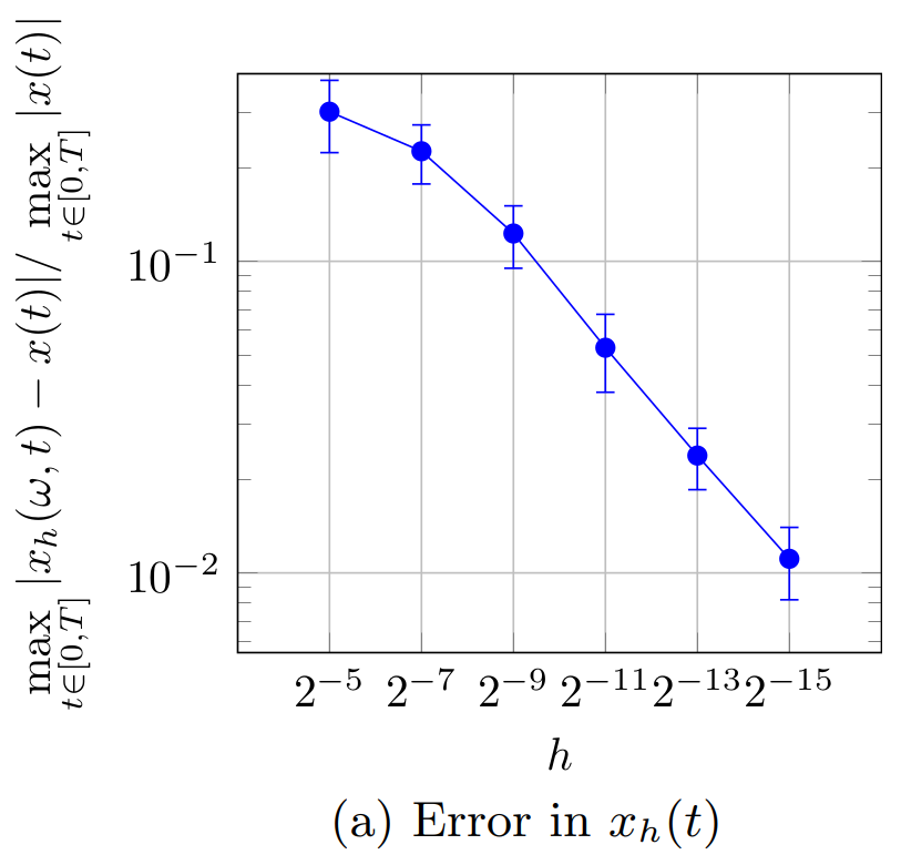
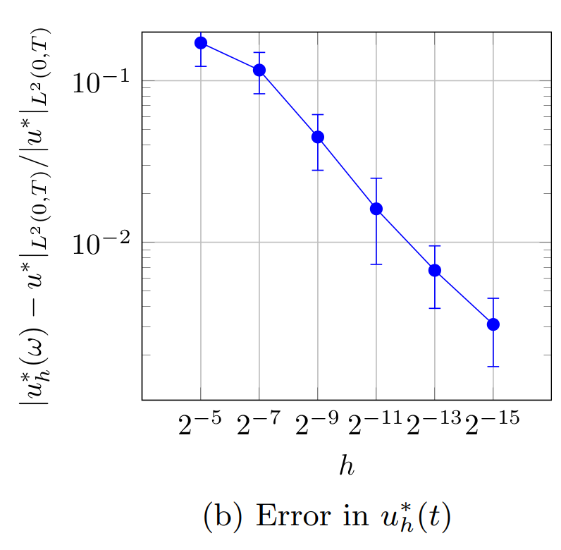
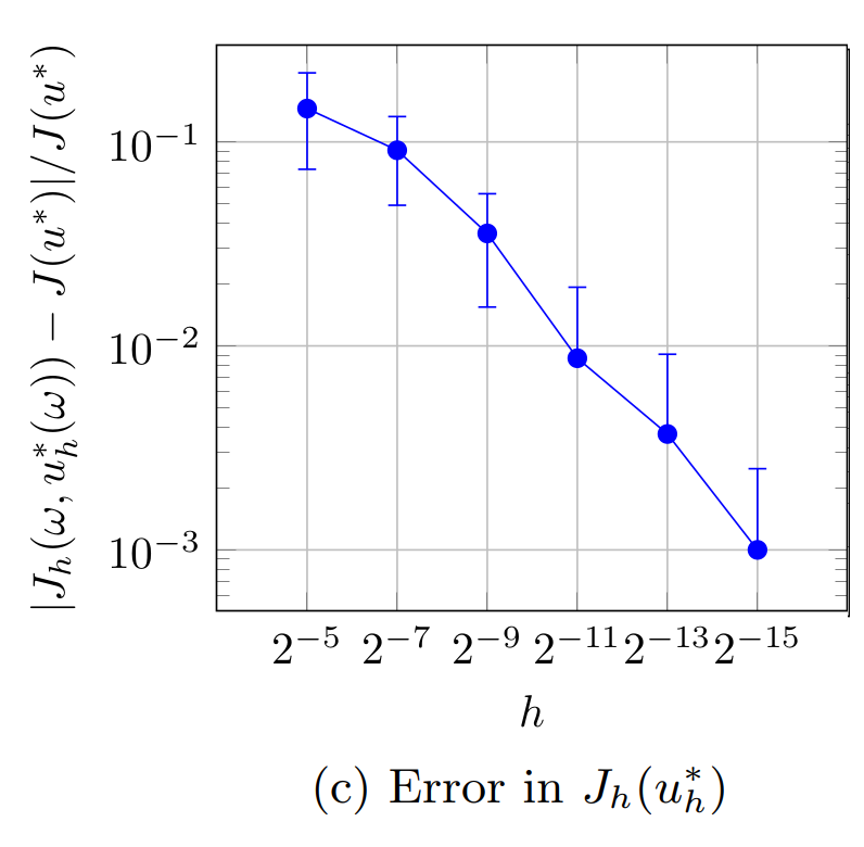
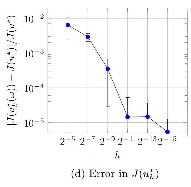
Figure 1. Simulation results for the discretized 1D heat equation
Figure 1b shows the difference |u_h^* - u^*|_{L^2(0,T)} between the optimal controls u^*(t) and u_h^*(\omega,t) that minimize (1) and (12), respectively. The average error is proportional to \sqrt{h}, which is the rate predicted by Main Result 4.
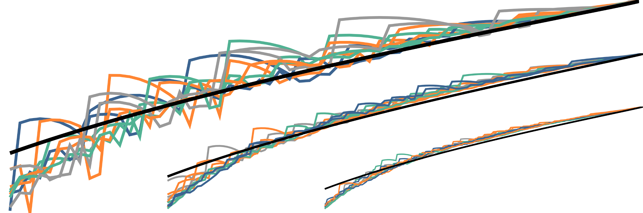
The convergence in the optimal controls in Figure 1b is also illustrated in Figure 2.
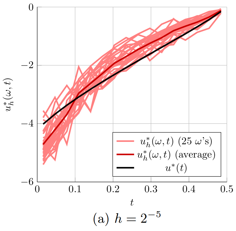
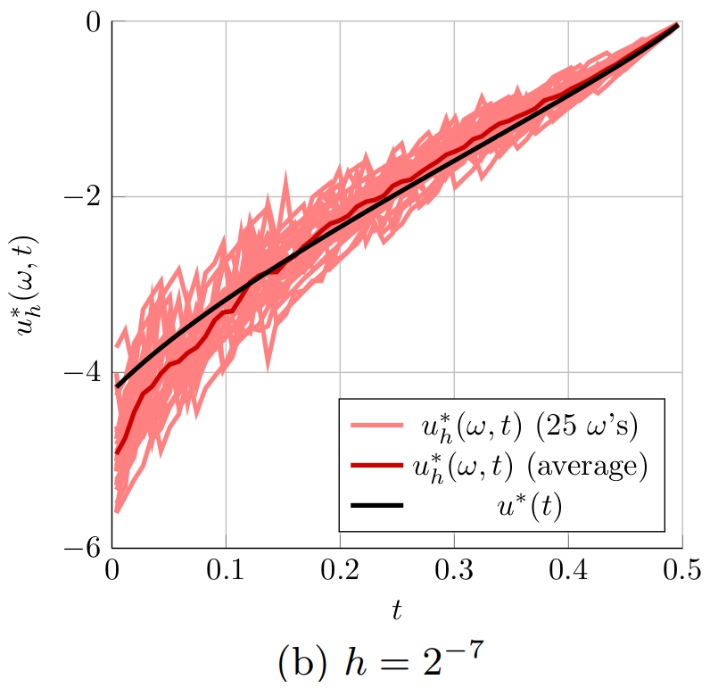
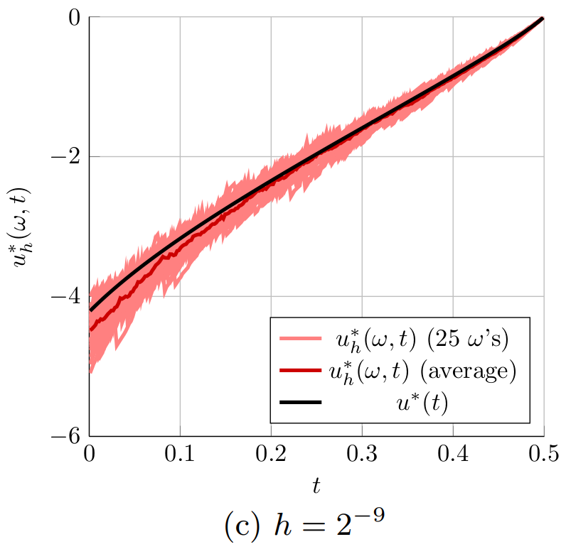
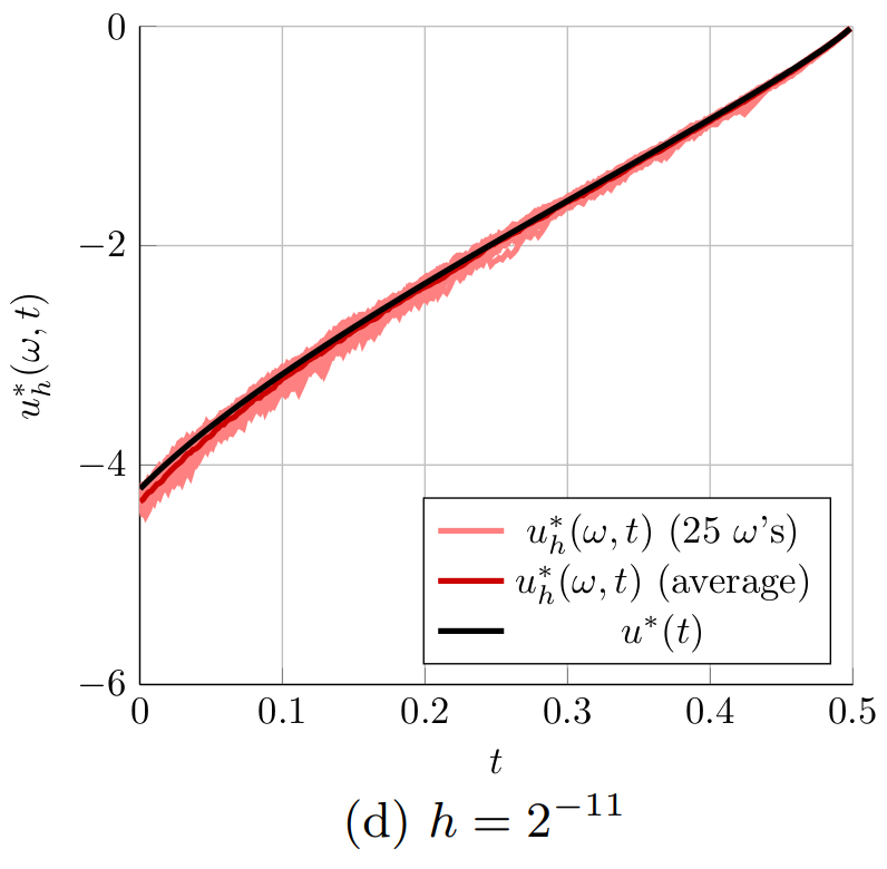
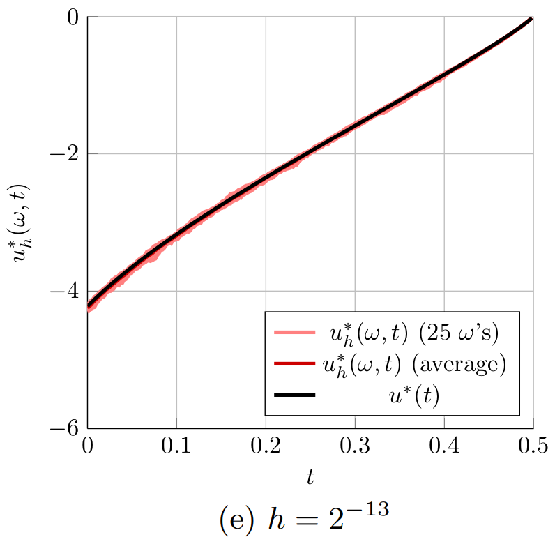
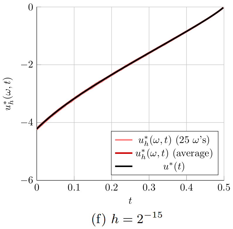
Figure 2. The optimal controls computed for the 1D heat equation for different time steps h. The controls u^*_h(\omega,t) computed with the proposed randomized time-splitting method are shown for 25 realizations of \omega and compared to the optimal control u^*(t) for the original system.
Figure 2 shows the optimal controls u_h^*(\omega,t) obtained for 25 randomly selected realizations of \omega \in \Omega (light red) for the six considered grid spacings h of the temporal grid. The figure also shows the average of the 25 optimal controls u^*_h(\omega,t) (dark red) and the optimal control u^*(t) for the original system (black). Figure 2 indeed shows that the optimal controls u_h^*(\omega,t) get closer to the optimal control u^*(t) when the spacing of the temporal grid h is reduced. Especially in Figures 2a and 2b, it is also clear that the average of the 25 optimal controls u^*_h(\omega,t) (dark red) is not equal to the optimal control u^*(t) for the original system (black). This indicates that \mathbb{E}[u_h^*] \neq u^*. This means that u^*_h is a biased estimator for u^* and averaging several realizations of u^*(\omega,t) can only improve the approximation of u^*(t) to a limited extend. Note, however, that
|\mathbb{E}[u_h^*] - u^*| = |\mathbb{E}[u_h^* - u^*]| \leq \mathbb{E}[|u^*_h - u^*|] \leq \sqrt{\mathbb{E}[|u^*_h - u^*|^2]},
so that the bound in Main Result 4 implies that \mathbb{E}[u_h^*] \rightarrow u^* as h \rightarrow 0.
Figures 1c and 1d illustrate the convergence of J_h(\omega,u^*_h(\omega)) and J(u^*_h(\omega)) to J(u^*). Figure 1c illustrates the error estimate in Main Result 3 and shows that the average difference |J_h(\omega,u^*_h(\omega)) - J(u^*)| is indeed proportional to \sqrt{h}. Figure 1d illustrates the error estimate in Main Result 5, which shows that the difference average |J(u_h^*(\omega)) - J(u^*)| is proportional to h. The convergence rate is now twice as high as in the previous cases and the relative error stabilizes around 10^{-5}, which seems to be related to the tolerance of 10^{-6} used in the computation of the optimal controls.
Because the considered system of ODEs is relatively small, the proposed stochastic splitting method does not lead to a reduction in computational cost for the considered problem. In other problems with a larger state dimension and denser A-matrices, we have observed a reduction in computational cost of a factor 2 to 3, see [9].
Conclusions and future research
-We have proposed a general framework for randomized time-splitting in LQ optimal control problems. The dynamics, the minimal values of the cost functional, and the optimal control obtained with the proposed randomized time-splitting method converge in expectation to their analogues in the original problem when the grid spacing of the time grid h goes to zero. The convergence rates in our theoretical results are also observed in the presented numerical example.
The presented results open several interesting directions for future research:
-We have presented results for infinite-dimensional systems, but our numerical results in [9] suggest that a similar approach can be used for in infinitedimensional systems. As the large literature on (deterministic) operator splitting also indicates, this extension is an interesting but challenging topic for future research.
-Another important topic for future research is the extension to nonquadratic cost functions constrained by nonlinear dynamics. This extension is particularly interesting because of the connections between the training of certain types of Deep Neural Networks (DNNs) and these types of optimal control problems, see, e.g., [3, 1, 4, 8], and is also important for the control of interacting particles systems, see [7].
-As suggested in [7], it is natural to combine the proposed randomized time-splitting method with a Model Predictive Control (MPC) strategy. An error analysis for this randomized MPC strategy not only involves the parameters h and Var[A_h] that characterize the proposed time-splitting method, but also the prediction and control horizons of the MPC strategy. Capturing the interaction between all these parameters is another challenging topic for future research.
References
[1] Martin Benning, Elena Celledoni, Matthias J. Ehrhardt, Brynjulf Owren, and Carola-Bibiane Schönlieb. Deep learning as optimal control problems: models and numerical methods. J. Comput. Dyn., 6(2):171–198, 2019. [2] L eon Bottou, Frank E. Curtis, and Jorge Nocedal. Optimization methods for large-scale machine learning. SIAM Rev., 60(2):223–311, 2018. [3] Weinan E. A proposal on machine learning via dynamical systems. Commun. Math. Stat., 5(1):1–11, 2017. [4] Carlos Esteve, Borjan Geshkovski, Dario Pighin, and Enrique Zuazua. Large-time asymptotics in deep learning, 2021. [5] Lars Grüne and Jürgen Pannek. Nonlinear model predictive control. Communications and Control Engineering Series. Springer, Cham, 2017. Theory and algorithms, Second edition [of MR3155076]. [6] Shi Jin, Lei Li, and Jian-Guo Liu. Random batch methods (RBM) for interacting particle systems. J. Comput. Phys., 400:108877, 30, 2020. [7] Dongnam Ko and Enrique Zuazua. Model predictive control with random batch methods for a guiding problem, 2020. [8] Domènec Ruiz-Balet and Enrique Zuazua. Neural ODE control for classification, approximation and transport, 2021. [9] Daniel W M Veldman and Enrique Zuazua. A framework for randomized time-splitting in linear-quadratic optimal control. Submitted, 2021.|| Go to the Math & Research main page


