
Mathematical modeling and numerical simulations for Gas Dynamics (on Networks)
 Sol G. Montero Carrasco
Gas transport networks are essential in the real world, e.g, energy supply, industrial applications, and emergency services. In our model, we focus on the gas flow of pipeline networks that are described by the Euler equations, which are given by a system of nonlinear partial differential equations (PDEs), which represent the motion of a compressible non-viscous fluid or a gas.
In this post, we begin by deriving the doubly nonlinear system from the Euler equations. We then model the spatial domain as a network, incorporating both transmission and boundary conditions pertinent to the system. Finally, to demonstrate the effectiveness of our approach, we present numerical simulations illustrating gas dynamics in different configurations: a single pipe, a tripod network, and a diamond-shaped network. These simulations highlight key features such as flow stability and the impact of boundary conditions, providing valuable insight into the behavior of gas networks under various conditions.
Modeling for gas flow on a single pipe
The transport of a compressible, non-viscous gas through a pipeline is described by the Euler equations, a system of nonlinear partial differential equations (PDEs) that ensure conservation of mass, momentum, and energy. The full set is given by see [3],[7],[10]. Let \rho denote the density, v the velocity of the gas, and p the pressure. Furthermore, the parameters are the cross-sectional area A, the diameter D, and the friction coefficient \lambda.
\partial_{t} \rho + \partial_{x} (\rho v) =0,
\partial_{t}(\rho v)+\partial_{x}\left(\rho v^{2}+ p\right) = -\frac{\lambda}{2 D}\rho v |v|. \hspace{0.3cm} (1)
The state variables of the system are \rho, the flux q=\rho \cdot v.
The speed of sound we denote as c, and we assume the diameter of the pipe and the speed of sound to be constant (i.e, |v| \ll c). We consider here the isothermal case only. Then, simplifying the momentum balance, our system (1) becomes,
\partial_{t} p+ \frac{c^{2}}{A}\partial_{x} q = 0, \hspace{0.3cm} (2)
\partial_{x}p^{2} = -\frac{\lambda c^{2}}{DA^2} q |q|, \hspace{0.3cm} (3)
Denoting by \delta=\frac{c}{A} and \alpha=\frac{\delta A}{c}, with \delta>0, \ \alpha>0. Equations (2)-(3) can be rewritten as,
\alpha\partial_{t} p+ \partial_{x} q = 0, \hspace{0.3cm} (4)
\partial_{x}p^{2} = -\delta^{2} q |q|. \hspace{0.3cm} (5)
Now, we set u(p)=p^{2}, then from (5) we deduce that
\partial_{x}u=-\delta|q| q,
and therefore, we have,
q=-\delta^{-1/2}\frac{\partial_{x}u}{|\partial_{x}u|^{1/2}}. \hspace{0.3cm} (6)
Substituting (6) in (4), we obtain the following doubly nonlinear system
\alpha\partial_{t}\left(\frac{u}{\sqrt{|u|}}\right)-\partial_{x}\left(\frac{\partial_{x}u}{|\partial_{x}u|}\right)=0. \hspace{0.3cm} (7)
By introducing the monotone function \beta(s):=\frac{s}{\sqrt{|s|}}, the system (7) can be rewritten in the compact form:
\alpha\partial_{t}\beta(u)-\partial_{x}\beta(\partial_{x} u)=0. \hspace{0.3cm} (8)
The equation (8) represents the gas flow in a single pipeline. In the next section, we will extend the model from studying a single edge of the network to multiple edges.
Network Modeling
In this section, we will introduce a network with multiple edges (pipes). Using conservation laws for mass and momentum, we can extend single-pipe models to networks, capturing key dynamics like pressure and flow interactions at junctions. These models are essential for optimizing design and operations in industries such as energy and transportation.
Definition 1.
Let \mathcal{G}=(V,E) be a finite directed graph.
• The outward-pointing normal n_{e}:V\rightarrow \{-1,0,1\} of an edge formed by v and [/katex]v’[/katex] (where v\neq v', i.e. e=(v,v') is defined by
n_{e}(v) = \begin{cases} -1, & \text{if the edge } e \text{ starts at node } v, \\ +1, & \text{if the edge } e \text{ ends at node } v', \\ 0, & \text{otherwise}. \end{cases}
• For any vertex v\in V,
E(v):=\{e\in E: e=(v,.) \ \text{or} \ e=(.,v')\},
is the set of adjacent edges.
• The set of vertices can be partitioned into,
V_{B}^{R} = \{v\in V \ : |E(v)|=1\},
V_{I} = \{v\in V \ : |E(v)|>1\},
where V_{B}^{R} is the set of boundary vertices and V_{I} is the set of interior vertices.
Now, we denote \mathcal{G}=(V,E,l) a metric graph, i.e. a directed graph with vertices V partitioned into boundary vertices V_{B}^{R} and interior vertices V_{I}, and with edges e\in E which are represented with intervals of length l_{e}. For clarity, we denote l_{e}=L>0, for all e\in E.
We define a function u:\mathcal{G}\rightarrow\mathbb{R} which identifies a function u_{e} for each edge e\in E.
To ensure the continuity of u at node v we can assume that
u_{e}(v,t)=u_{e'}(v,t),\quad \forall\ v\in V_{I} , \text{and} \ e,e'\in E(v). \hspace{0.3cm} (9)
On the other hand, we will assume that the flux is continuous. This can be formulated using the following the Kirchhoff-type condition,
\sum_{e\in E} a_{e}(v)\beta(\partial_{x}u_{e}(v,t))n_{e}(v), \quad v\in V_{I}=0 . \hspace{0.3cm} (10)
where a_{e}(v):=|E(v)| the number of edges that incidence the vertex v.
We assume a Robin boundary conditions in vertices V_{B}^{R} is given as follows:
\delta^{-1/2}\beta(\partial_{x}u_{e}(v,t))n_{e}(v)=\gamma(\beta(u_{e}(v,t))-g_{v}),\quad v\in V_{B}^{R}, \hspace{0.3cm} (11)
where
• \delta>0 is a stability term.
• \gamma is a scalar parameter.
• g_{v} is a boundary term specified to each vertex v\in V_{B}^{R}, representing a constant or predefined value at the vertex.
On the domain for each edge e\in E, \{\ (x,t) \ | \ 0\le t\le T, 0 \lt x \lt l_{e}\} we consider for system (8) with the initial condition
t=0:~ u_{e}(x,t)=u^{e}_{0}, \quad e\in E, \ x\in (0,l_{e}). \hspace{0.3cm} (12)
We summarize the equations as follows, over the time interval (0,T) (see e.g. Leugering et al. [6]} and Schöbel-Kröhn [9]),
\begin{cases} \alpha\partial_{t}\beta(u_{e}(x,t))-\partial_{x}\beta(\partial_{x} u_{e}(x,t))=0, \quad e\in E, x\in (0,L),\\\\ u_{e}(v,t)=u_{e'}(v,t), \quad v\in V_{I},\, e,e'\in E\\\\ \sum_{e\in E} a_{e}(v)\beta(\partial_{x}u_{e}(v,t))n_{e}(v)=0, \quad v\in V_{I}.\\\\ \delta^{-1/2}\beta(\partial_{x}u_{e}(v,t))n_{e}(v)=\gamma(\beta(u_{e}(v,t))-g),\quad v\in V_{B}^{R},\, e\in E,\\\\ u_{e}(x)=u^{0}_e(x), \quad e\in E,\, x\in (0,L). \end{cases} \hspace{0.3cm} (13)
Example 1.
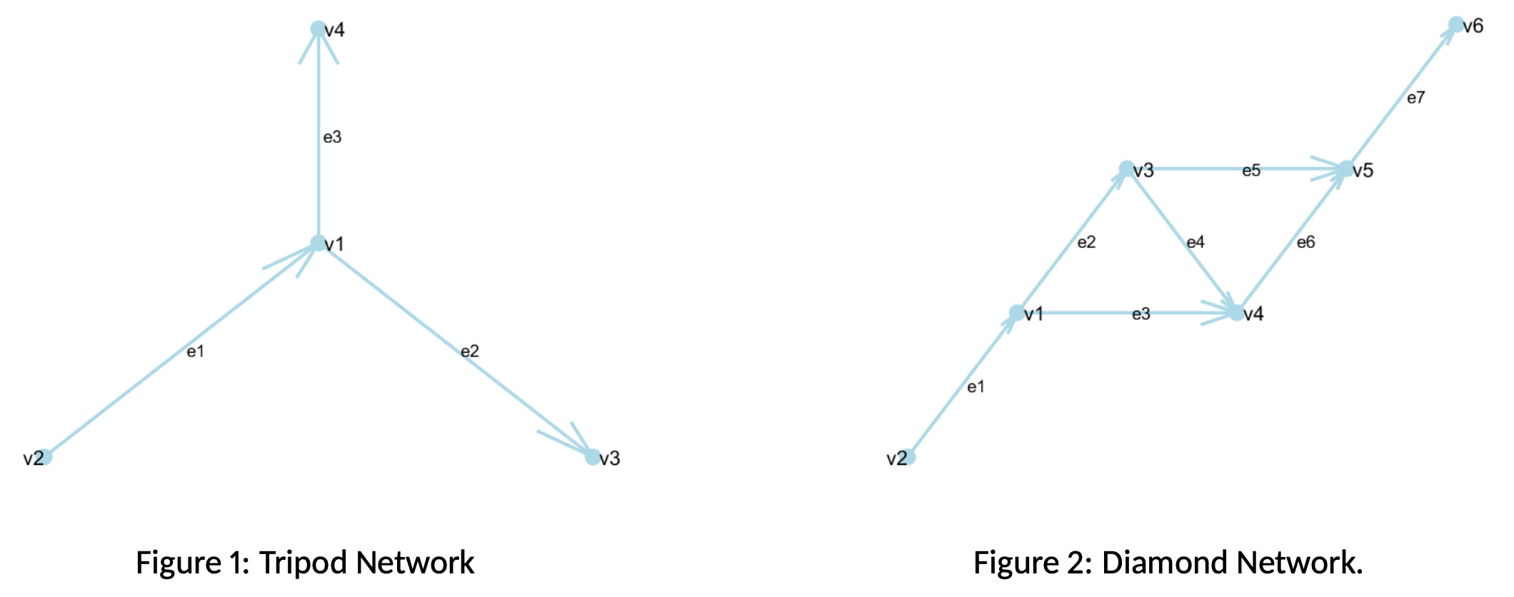
Consider a directed graph \mathcal{G}=(V,E) shown as Figure 1.
The set of edges E=\{e_{1},e_{2},e_{3}\} and vertices V=\{v_{1},v_{2},v_{3},v_{4}\}.
The edges are given by the vertex tuples e_{1}=(v_{2},v_{1}), e_{2}=(v_{1},v_{3}) and e_{3}=(v_{1},v_{4}).
Hence, v(e_{1})=\{v_{2},v_{1}\}, v(e_{2})=(v_{1},v_{3}) and v(e_{3})=\{v_{1},v_{4}\}.
For each vertex the adjacent edges are E(v_{1})=\{e_{1},e_{2},e_{3}\}, E(v_{2})=\{e_{1}\}, E(v_{3})=\{e_{2}\} and E(v_{4})=\{e_{3}\}.
The interior and boundary vertices V_{I}=\{v_{1}\} and V_{B}^{R}=\{v_{i}\}_{i=2}^4.
The non-zero values of the outward-pointing normals are n_{e_{1}}(v_{1})=n_{e_{3}}(v_{4})=n_{e_{2}}(v_{3})=1 and n_{e_{1}}(v_{2})=n_{e_{2}}(v_{1})=n_{e_{3}}(v_1)=-1.
Numerical results
We explore the behaviour of a pipeline network, starting with the simplest model, a single pipe, and extend it to different structures, such as the Tripod Network and Diamond network [8]. To discretize in space our system we use the Finite Element Method (FEM) and to discretize in time we apply Implicit Euler Method.
Single pipe
The simplest form of gas transportation is through a single pipeline, which is considered a general two-point boundary value problem. Recalling the development of the explicit mathematical model for gas flow dynamics in a pipeline in Leugering et al. [6]. We created a Matlab program from scratch and material used from Jin Liu [8]. The modeling is based on several assumptions:
• The gas flow is assumed to be along a single spatial dimension, and any changes in crosssectional area along the pipeline are gradual.
• Horizontal pipeline, where the radius of curvature is large. But its diameter stays constant, for simplifications in the flow equations.
• The velocity and the temperature are considered constant along the length of the pipe.
With these assumptions, a single pipeline e\in E is described by the system (13).
Tripod Network and Diamond Network
In this case, for the Tripod network, we assume that the gas flows through one entry pipe and exits through two pipes (or vice versa). We need to ensure a proper gas flow modeling we need to consider the assumptions as the single pipe model and that there is no vacuum present, the gas density \rho_{e_{i}}>0 ensures that the flow is subsonic making the flow stable and realistic for real-world pipelines. We consider that the friction is inside only in each pipe e_{i}, which only affects the gas flow through the pipes, not the junctions. Although in this model we need to establish coupling conditions at the junction (in Figure 1 node v_{1} where multiple edges meet).
In the second example, the Diamond Network, it is a circle network which consists of seven oriented pipes connected as in Figure 2, that splits the gas flow at a junction point, and then the branches connect again in a single pipe.
Both networks are modeled by the nonlinear parabolic system (13).
Simulation Setting
In our system (13) we have a Robin boundary condition. However, we can also impose a Dirichlet or Neumann
boundary condition depending on the values of our parameters \gamma and g. We have three cases:
1. Neumann Boundary Condition: if we consider \gamma=0.
2. Robin Boundary Condition: if \gamma\neq 0 and does not tend to infinity.
3. Dirichlet Boundary Condition: for \gamma large, when \beta(u(x,t))\neq g, there is mass flux between the pipeline and the ambient medium. As \gamma tends to infinity, the Robin boundary approximates the Dirichlet condition \beta(u(x,t))=g.
For our numerical simulations, we solve our nonlinear equation using the Finite Element Method (FEM), adapted to handle the nonlinearity of the problem through an iterative scheme. We use 200 time steps and 200 spatial steps for the discretization. The main parameters for the simulation are: edge length L = 1 , \alpha = 1 , and \delta= 10^{-6}. The initial condition is u(x, 0) = \sin^2(\pi x) . For the FEM method, we set the following boundary conditions:
For the FEM method, we set the following boundary conditions:
• Neumann boundary: \gamma= [0 \,, 0] and g=[1 \,, 1].
• Robin boundary: \gamma= [1 \,, 1] and g=[0 \,, 0].
• Dirichlet boundary: \gamma= [10^6\,, 10^6] and g=[0 \,, 0].
Finally, we compare the results obtained with the FEM algorithm to those generated by MATLAB’s ‘pdepe ‘ function, which approximates the solution to the PDE numerically.
Single-pipe simulation
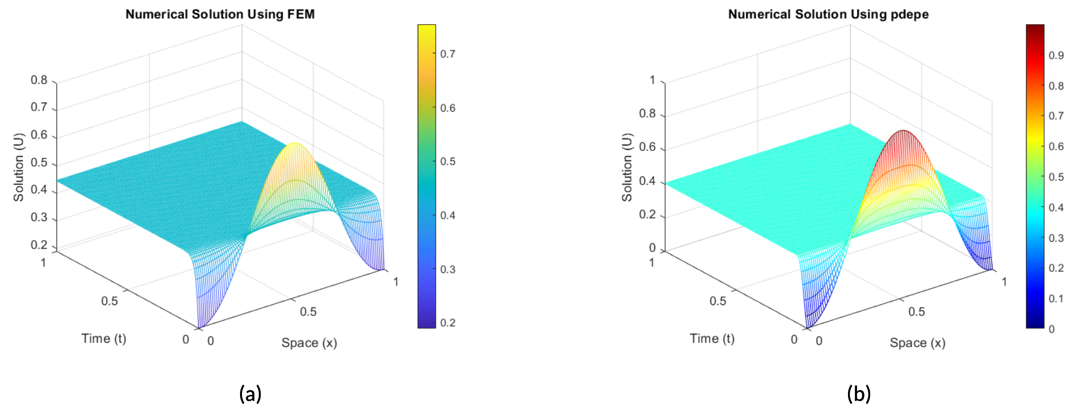
Figure 3. Gas Flow Simulation on Single Pipeline [0,L] with Neumann boundary condition.
In (a) we illustrate the numerical simulation using FEM. In (b), we illustrate the numerical simulation using the pdepe function.
First, we simulate the gas flow through a single pipe with the Neumann boundary condition. This condition implies that there is no flux across the boundary, which means that the gradient of the solution at the boundary is zero. We observed that it verifies the zero Neumann condition and that both methods in Figures 3a and 3b capture the expected behavior under the Neumann condition
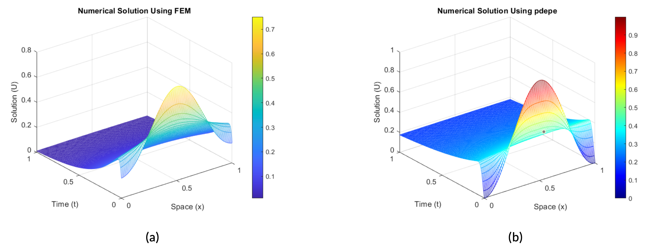
Figure 4. Gas Flow Simulation on Single Pipeline [0,L] with Robin boundary condition.
In (a) we illustrate the numerical simulation using FEM.
In (b), we illustrate the numerical simulation using the pdepe function.
In Figures 4b and 4a we show a simulation with Robin boundary conditions, which combines Dirichlet and Neumann boundary conditions. The results shows the gas flow behavior under these conditions, with the FEM results
closely matching the pdepe simulations. Also, the wave amplitude diminishes as time increases, and the solution seems to stabilize, indicating a dissipative system.
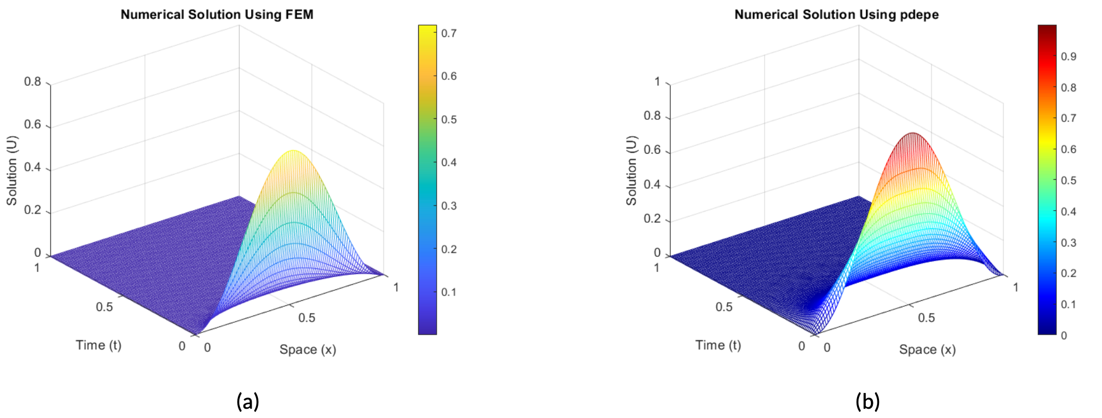
Figure 5. Gas Flow Simulation on Single Pipeline [0,L] with Dirichlet boundary condition.
In (a) we illustrate the numerical simulation using FEM.
In (b), we illustrate the numerical simulation using the pdepe function.
Finally, in Figures 5b and 5a we show a Dirichlet boundary condition simulation. The Dirichlet condition assumes that the solution is fixed at the boundary. Then, as \gamma increases, the Robin boundary approximates the Dirichlet condition, forcing the solution to a fixed value at the boundary. Therefore, the comparison of the illustrations shows how the gas stabilizes when the boundary values are fixed.
Tripod network simulation
In this case, we consider analogously the setting parameters as the single pipeline, but for the boundary condition, we have three boundary condition cases. Also, for the initial condition for each pipe e_{i} we need to consider u_{e_{i}}(0)=u_{e_{j}}(0) for i,j=1,2,3 and u_{e_{i}}(1)=0 for i=1,2,3. We have the following animation for each different scenario (Neumann, Dirichlet, and Robin boundary conditions):
In our tripod simulations, we first simulate our model with a Dirichlet boundary condition. We observe that while the time step increases, the value of the boundary is fixed to zero, and the solution tends to stabilize to zero.
Secondly, we simulate for Neumann boundary conditions and we observe that when the time step increases, the pipes start to level off and become a more stable system. At the end, the pipes are flattened, with a smaller amplitude, and our system has stabilized. To conclude, we simulate our system with both boundary conditions (Dirichlet and Neumann), i.e, with Robin boundary condition. Then, with a mixed boundary condition, we note that over the evolution of time, we observe a smoother transition between the curves, and it stabilizes the system.
Diamond Network simulation
In the simulation, we set the same setting as for the single pipeline. We apply only Robin boundary simulation, as we have observed before Dirichlet and Neumann boundary conditions, then our model will have the same evolution in time as the Tripod network, but with a different graph model. Then, we show the diffusion results of the whole system. We observe in this model that when the time step increases our solution stabilizes to zero.
Conclusions
In conclusion, this study presents a mathematical model for gas transport in pipeline networks, focusing on the nonlinear hyperbolic systems that govern fluid motion. Through the use of Finite Element Method (FEM) and Backward Euler Method for numerical discretization, simulations of gas flow were performed for different network configurations: a single pipe, a tripod, and a diamond network. The results for various boundary conditions (Neumann, Dirichlet, and Robin) demonstrate how the flow stabilizes under different setups. These simulations illustrate the dynamic behavior of gas flow and provide insights into real-world applications of gas transport networks.
Note that in Egger et al. [4], it is shown that discrete solutions converge exponentially to their steady states when the boundary data remains constant. However, the rate of stabilization is influenced not only by the boundary data but also by the topology of the pipeline network. Well-connected networks tend to stabilize faster than sparsely connected ones, as flow redistribution plays a key role in achieving equilibrium.
Future research could explore higher-order numerical schemes, adaptive mesh refinement, and control strategies to further enhance the efficiency and stability of pipeline network simulations.
I would like to acknowledge the support and motivation provided by my supervisor Yue Wang, Martin Hernandez Salinas, and Jin Liu, whose contributions have been invaluable throughout this process and I want to thank for this opportunity to Enrique Zuazua Iriondo.
References
[1] W. Arendt and W. Mahamadi (2003) The laplacian with robin boundary conditions on arbitrary domains. Mathematics Subject Classifications, Vol. 19, pp. 47–54[2] George Keith Batchelor (2000) An introduction to fluid dynamics. Cambridge university press
[3] J. Brouwer, I. Gasser, M. Herty (2011) Gas pipeline models revisited: Model hierarchies, nonisothermal models, and simulations of networks. Multiscale Modeling and Simulation, Vol. 9, pp. 601–623.
[4] H. Egger and J. Giesselmann (2023) Regularity and long time behavior of a doubly nonlinear parabolic problem and its discretization, Vol. 5
[5] G. Leugering (2022) Nonoverlapping domain decomposition for instantaneous optimal control of friction dominated flow in a gas-network. Technical report, Friedrich-Alexander-Universität Erlangen-Nürnberg
[6] G. Leugering and G. Mophou (2010) Instantaneous optimal control of friction dominated flow in a gas-network. Technical report, Friedrich-Alexander-Universität Erlangen-Nürnberg
[7] R J. LeVeque (2012) Finite volume methods for hyperbolic problems. Cambridge University Press
[8] Jin Liu (2022) Domain decomposition of frictional dominated flow in a gas network. Master’s thesis, FriedrichAlexander-Universität Erlangen-Nürnberg
[9] L. Schöbel-Krön (2020) Analysis and numerical approximation of nonlinear evolution euqations on network structures
[10] J. Smoller (1983) Waves and Reaction-Diffusion Equations, Vol. 258. Springer Verlag.
[11] W. A. Strauss (2007) Partial Differential Equations (An Introduction). John Wiley and Sons
|| Go to the Math & Research main page


