
Daniel Veldman, FAU DCN-AvH
Code: ![]() || Also available @Daniël’s GitHub
|| Also available @Daniël’s GitHub
In a previous post “Randomized time-splitting in linear-quadratic optimal control“, it was proposed to use the Random Batch Method (RBM) to solve classical Linear-Quadratic (LQ) optimal control problems. This contribution is concerned with the corresponding numerical implementation.
We thus consider the classical LQ optimal control problem, in which the goal is to find the control u(t) that minimizes
J(u) = \frac{1}{2}\int_0^T \left( (x(t)-x_d(t))^\top Q (x(t)-x_d(t))+u(t)^\top R u(t) \right) \ \mathrm{d}t,
subject to the dynamics
\dot{x}(t) = Ax(t) + Bu(t), \qquad \qquad x(0) = x_0.
Here, x(t) and x_d(t) evolve in \mathbb{R}^N and u(t) evolves in \mathbb{R}^q. When N is large, this problem is typically solved by a gradient-based algorithm such as gradient descent or conjugate gradients. The gradients required in these algorithms can be computed efficiently as
(\nabla J(u))(t) = B^\top \varphi(t) + R u(t),
where the adjoint state \varphi(t) satisfies
-\dot{\varphi}(t) = A^\top \varphi(t) + Q (x(t) - x_d(t)), \qquad \qquad \varphi(T) = 0.
Note that the adjoint state \varphi(t) can be computed by integrating backward in time starting from the final condition \varphi(T) = 0. Also note that x(t) in the ODE for \varphi(t) is the solution of the state equation in which the input u(t) represents the point in which the gradient is computed. This means that both the forward dynamics for x(t) and the backward dynamics for \varphi(t) need to be solved at every iteration. Furthermore, a numerical implementation of the above procedure requires time-discretization of the above equations. This will be discussed in more detail below. Note that this approach is computationally demanding when A is large and not sparse and when there is a large number of points in the time grid.
The RBM can be used to speed up the computation of the minimizer u^*(t). To apply the RBM, the matrix A is written as the sum of M submatrices A_m
A = \sum_{m=1}^M A_m.
To gain a computational advantage of the proposed method, the submatrices A_m should typically be more sparse than the original matrix A. It is also advantageous to choose the submatrices A_m dissipative when possible. The time interval [0,T] is then divided into K subintervals [t_{k-1}, t_k). The idea of the proposed method is to consider a random subset of the matrices A_m in each time interval. To make this precise, the 2^M subsets of \{1,2, \ldots, M \} are denoted by S_1, S_2, \ldots S_{2^M}. To every subset S_\ell (\ell \in \{1, 2, \ldots , 2^M \}) a probability p_\ell is assigned. The probabilities p_\ell should satisfy
\sum_{\ell = 1}^{2^M} p_\ell = 1,
and enable us to compute the probabilities
\pi_m = \sum_{\ell \in \mathcal{L}_m} p_\ell, \qquad \qquad \mathcal{L}_m = \{ \ell \in \{1,2, \ldots, 2^M \} \mid m \in S_\ell \}.
Note that the \pi_m is the probability that an index m is an element of the selected subset.
For each of the K time intervals [t_{k-1},t_k), an index \omega_k \in \{1,2, \ldots , 2^M \} is selected according to the chosen probabilities p_\ell. The selected indices form a vector
\boldsymbol \omega := (\omega_1, \omega_2, \ldots , \omega_K) \in \{1,2,\ldots ,2^M \}^K =: \Omega.
The selected \boldsymbol \omega \in \Omega defines a piece-wise constant matrix t \mapsto A_h(\boldsymbol \omega,t)
A_h(\boldsymbol \omega, t) = \sum_{m \in S_{\omega_k}} \frac{A_m}{\pi_m}, \qquad \qquad t \in [t_{k-1}, t_k).
Note that this formula shows that the probabilities p_\ell should be chosen such that \pi_m > 0 for all m \in \{ 1,2, \ldots, M \}.
Instead of solving the original optimal control problem that involves the (typically large and not sparse) matrix A, it is proposed to find the optimal control u^*_h(\boldsymbol \omega, t) that minimizes
J_h(\boldsymbol \omega, u) = \frac{1}{2}\int_0^T \left( (x_h(\boldsymbol \omega,t)-x_d(t))^\top Q (x_h(\boldsymbol \omega,t)-x_d(t))+u(t)^\top R u(t) \right) \ \mathrm{d}t,
subject to the dynamics
\dot{x}_h(\boldsymbol \omega,t) = \mathcal{A}_h(\boldsymbol \omega,t) x_h(\boldsymbol \omega,t) + B u(t), \qquad \qquad x_h(\boldsymbol \omega,0) = x_0.
The optimal control u_h^*(\boldsymbol \omega,t) is again typically computed by a gradient-based algorithm in which the gradient is computed as
\nabla J_h(\boldsymbol \omega, u) = B^\top \varphi_h(\boldsymbol \omega, t) + R u(t),
where \varphi_h(\boldsymbol \omega, t) satisfies
-\dot{\varphi}_h(\boldsymbol \omega, t) = (A_h(\boldsymbol \omega, t))^\top \varphi(\boldsymbol \omega, t) + Q(x_h(\boldsymbol \omega,t) - x_d(t)), \qquad \varphi_h(\boldsymbol \omega, T) = 0.
Note that the randomized optimal control problem is typically more easy to solve than the original problem because the matrix A_h(\boldsymbol \omega, t) is more sparse than the original matrix A. Also note that the vector of randomized indices \boldsymbol \omega is kept fixed during the optimization process. As explained in the previous post, the functions x_h(\omega,t) and u_h^*(\boldsymbol \omega,t) converge in expectation to the solutions of the original problem x(t) and u^*(t) as the grid spacing of the temporal grid h approaches zero. In particular, the probability that the distance u^*_h(\boldsymbol \omega, t) - u^*(t) is larger than some \varepsilon > 0 approaches zero when h \rightarrow 0.
We discretize the forward dynamics for x_h(\boldsymbol \omega, t) by the Crank-Nicholson scheme, the cost functional J_h(\boldsymbol \omega, u) by a combination of the trapezoid rule and the midpoint rule, and the backward dynamics for \varphi_h(\boldsymbol \omega, t) by the scheme proposed in [1] that leads to the exact gradient of the discretized cost functional. because u^*_h(\boldsymbol \omega, t ) is a better approximation of u^*(t) when h is smaller, the time intervals [t_{k-1}, t_k) used in the RBM coincides with the grid for the time discretization.
The matlab code for three numerical examples from [3] can be downloaded from this page. The following three problems are addressed in these examples:
• A finite difference discretization of the optimal control problem in which
\mathcal{J}(u) = \frac{100}{2}\int_0^T \int_{-L}^0 y(t,\xi)^2 \ \mathrm{d}\xi \ \mathrm{d}t + \frac{1}{2}\int_0^T u(t)^2 \ \mathrm{d}t.
is minimized subject to the heat equation
\begin{aligned}
&y_t(t,\xi) = y_{\xi\xi}(t,\xi) + \chi_{[-L/3,0]}(\xi) u(t), \qquad \xi \in [-L,L], \\
&y_\xi(t,-L) = y_\xi(t,L) = 0, \qquad \qquad y(0,\xi) = e^{-\xi^2} + \xi^2e^{-L^2}.
\end{aligned}
The splitting of the operator A is based on a decomposition of the spatial domain [-L, L] into M intervals of equal length.
• A finite difference discretization of the optimal control problem in which
\mathcal{J}(u) = 1000 \int_0^T \iint_{S_{\mathrm{side}}} (y(t,\boldsymbol \xi))^2 \ \mathrm{d}\boldsymbol \xi \ \mathrm{d}t + \int_0^T (u(t))^2 \ \mathrm{d}t,
is minimized subject to the 3-D heat equation
\begin{aligned} &y_t(t,\boldsymbol \xi) = \Delta y(t, \boldsymbol \xi), \qquad\qquad\qquad & \boldsymbol \xi \in [-L,L]^3, \\ &\nabla y(t,\boldsymbol \xi) \cdot \mathbf{n} = u(t), \qquad \qquad\qquad & \boldsymbol \xi \in S_{\mathrm{top}}, \\ &\nabla y(t,\boldsymbol \xi) \cdot \mathbf{n} = 0, \qquad \qquad\qquad & \boldsymbol \xi \in \partial V \backslash S_{\mathrm{top}}, \\ &y(0,\boldsymbol \xi) = e^{-\lvert \boldsymbol \xi \rvert^2/(8L^2)}, \end{aligned}
where S_{\mathrm{side}}= \{ \xi_1 = -L \} and S_{\mathrm{top}} = \{ \xi_3 = L \}.
The splitting of the operator A is now based on a random splitting of the interactions between the different nodes in the finite difference grid.
• A finite element discretization of the optimal control problem in which
\mathcal{J}(u) = \frac{100}{2}\int_0^T \int_{-L}^L y(t,\xi)^2 \ \mathrm{d}\xi \ \mathrm{d}t + \frac{1}{2}\int_0^T \left( (u_1(t))^2 + (u_2(t))^2 \right) \ \mathrm{d}t,
is minimized subject to the fractional heat equation
\begin{aligned}
&y_t(t,\xi) = -(-d_\xi^2)^sy(t,\xi) + \chi_{[-L/3,0]}(\xi) u_1(t) + \chi_{[L/3,2L/3]}(\xi) u_2(t), \\
&y(t,-L) = y(t,L) = 0, \qquad \qquad y(0,\xi) = e^{-\beta^2\xi^2} - e^{-\beta^2L^2}.
\end{aligned}
The finite element discretization is based on [2].
The splitting of the operator A is now obtained by dividing A into P \times P blocks.
These problems and their discretization are described in more detail in [3]. A discussion on the theoretical underpinning of the proposed method can be found in a previous post (insert link) and in [3].
The code can be executed by running the files example1 heat1D, example2 heat3D, and example3 fractional3D. Figures 1, 2, and 3 show the typical results. Note that the specific plots depend on the randomly selected vector of indices \boldsymbol \omega, and that the specific solutions will be different every time than the files are executed.
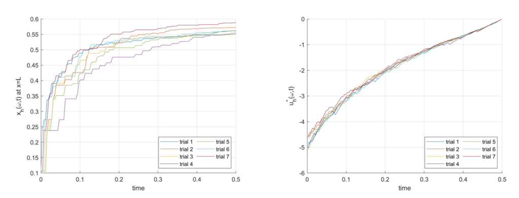
Figure 1. One coefficient of x_h(ω, t) and the optimal control u^∗_h (ω, t) for 7 realizations of ω for Example 1, obtained by running example1 heat1D.
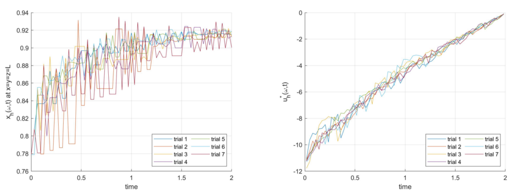
Figure 2. One coefficient of x_h(ω, t) and the optimal control u^*_h (ω, t) for 7 realizations of ω for Example 2, obtained by running example2 heat3D.
These problems and their discretization are described in more detail in [3]. A discussion on the theoretical underpinning of the proposed method can be found in a previous post (insert link) and in [3].
The code can be executed by running the files example1 heat1D, example2 heat3D, and example3 fractional3D. Figures 1, 2, and 3 show the typical results. Note that the specific plots depend on the randomly selected vector of indices ω, and that the specific solutions will be different every time than the files are executed.
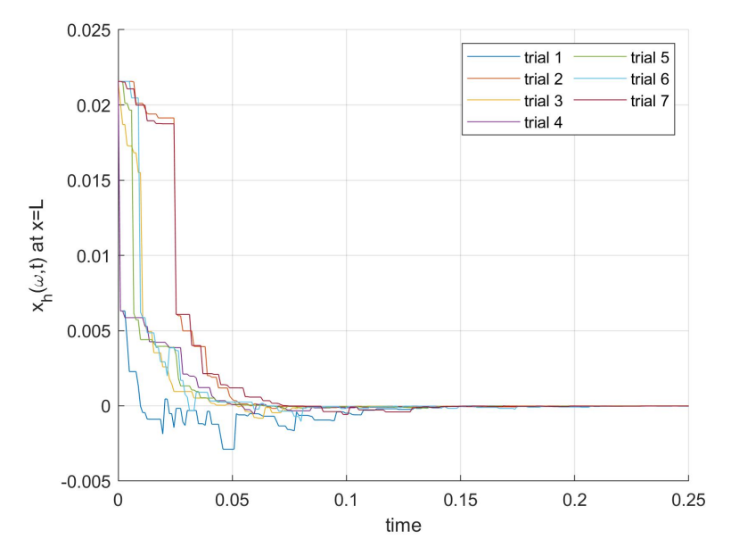
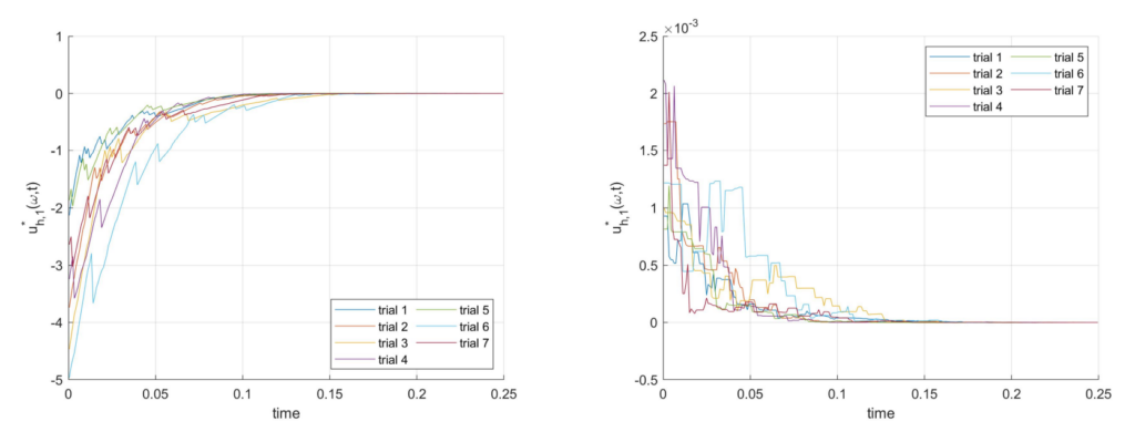
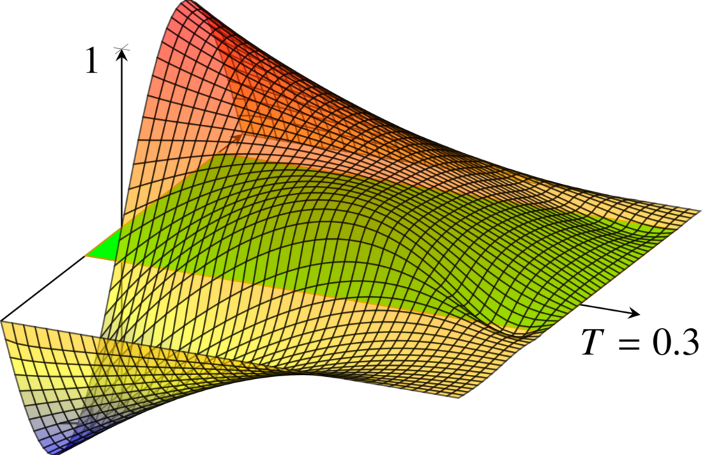
Figure 3. One coefficient of x_h(ω, t) and the optimal control u^*_h (ω, t) for 7 realizations of ω for Example 3, obtained by running example1 fractional1D.
References
[1] Thomas Apel and Thomas G. Flaig. Crank-Nicolson schemes for optimal control problems with evolution equations. SIAM J. Numer. Anal.,50(3):1484–1512, 2012.[2] Umberto Biccari and Víctor Hernández-Santamaría. Controllability of a one-dimensional fractional heat equation: theoretical and numerical aspects. IMA Journal of Mathematical Control and Information, 36(4):1199–1235, 07 2018.
[3] Daniel W M Veldman and Enrique Zuazua. A framework for randomized time-splitting in linear-quadratic optimal control. In preparation, 2021.
Code: ![]() || Also available @Daniël’s GitHub
|| Also available @Daniël’s GitHub
|| Go to the Math & Research main page


