
 Giulia Sambataro in collaboration with
Multi-physics problems, involving coupled phenomena such as fluid mechanics, thermodynamics, and chemistry, are common in science and engineering. These problems often involve distinct governing equations (e.g., Navier–Stokes, elasticity, diffusion) and specialized solvers, making monolithic solutions computationally prohibitive. Domain decomposition (DD) offers an effective strategy by partitioning the domain into subregions with localized models, which are then coupled to approximate the global solution. In many applications—e.g., geophysics, radioactive waste management, and mining—high-fidelity models (based on partial differential equations (PDEs)) are either unavailable or too costly to simulate: this fact motivates the use of machine learning (ML) surrogates. Data-driven models can be thus employed to capture complex, nonlinear dynamics from experimental data and support prediction and uncertainty quantification.
In this post I present a preliminary hybrid framework for solving steady multi-fidelity problems by:
(i) decomposing the domain into non-overlapping subdomains;
(ii) assigning PDE-based or ML-based local models to each subdomain; and
(iii) coupling subdomains through a data-driven adapted versions of the classical Dirichlet–Neumann algorithm.
The final goal is to develop a rigorous and modular theory enabling seamless integration of multi-fidelity, multi-physics components.
1 Non overlapping domain decomposition
We consider a domain \Omega \subset \mathbb{R}^d (with d=2) with Lipschitz boundary \partial \Omega and x \in \bar{\Omega} a space variable. We also consider a Hilbert space \mathcal{X}= [H_0^1(\Omega)]^d endowed with the norm \|v\|_{\mathcal{X}}:=\|v\|_{H^1(\Omega)}.
We consider a non-overlapping decomposition of \Omega into N_{\rm dd} subdomains
\Omega = \bigcup_{i=1}^{N_{\text{dd}}} \overline{\Omega}_i, \quad \Omega_i^\circ \cap \Omega_j^\circ = \emptyset \quad \text{for } i \ne j,
The interface \Gamma is defined as \Gamma := \partial \Omega_1 \cap \partial \Omega_2 and the trace operator is denoted as \gamma : H^1(D) \to H^{1/2}(\Gamma) for all D \subset \mathbb{R}^d (we use the same notation for the trace operator on the global domain \Omega and on its subdomains \Omega_i).
We denote as \Gamma_{i,\rm{dir}} \subset \partial \Omega_i \setminus \Gamma the local Dirichlet boundaries.
We introduce the following spaces
\mathcal{X}_i=\{v|_{\Omega_i}, v \in \mathcal{X}\}= [H^1(\Omega_i)]^d , \; \mathcal{X}_{i,0}=\{v \in \mathcal{X}_i \, | \, v =0 \, \text{at} \, \Gamma_{i,\rm{dir}}\}, \; \mathcal{U}=[L^2(\Gamma)]^d
We equip the Hilbert spaces \mathcal{X}_i with the norms \|v\|_{X_i}=\|v\|_{H^1(\Omega_i)} for i=1, \ldots, N_{\rm dd} and \|g\|_{\mathcal{U}}=\|g\|_{L^2(\Gamma)}.
We consider finite elements discretizations of the domains and we denote as N^{\rm hf}_i the degrees of freedom of finite element vectors in each subdomain i=1, \ldots, N_{\rm dd}.
2 A Dirichlet-Neumann scheme for multi-fidelity coupling
We present the methodology for N_{\rm dd}=2 subdomains which we denote as \Omega_{\rm{phys}} and \Omega_{\rm{data}}; they are associated with indices 1 and 2 of the general notation, respectively. We couple a physics-based model in \Omega_{\text{phys}} with a data-driven one in \Omega_{\text{data}}: for the latter, we use noisy measurements available at n_{\text{sample}} locations on \Gamma or on the subdomain \Omega_{\rm{data}}.
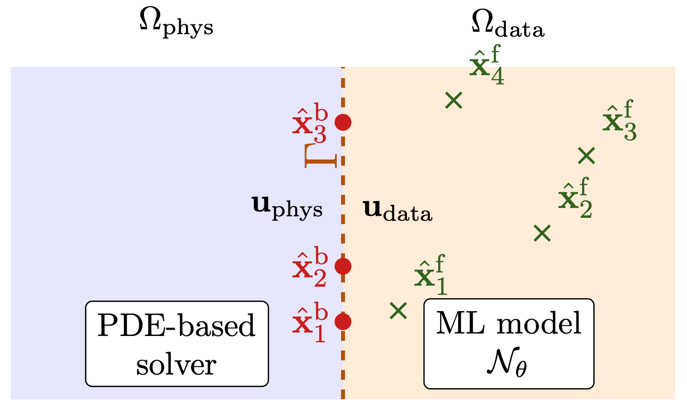
Figure 1. Schematic of the Physics–Data Interface Coupling: information is exchanged across the interface \Gamma.
The training dataset is given by:
\mathcal{D} = \left\{(\hat{\mathbf{x}}_i, \mathbf{u}^{\text{sample}}_i)\right\}_{i=1}^{n_{\text{sample}}} \quad \text{with} \quad \mathbf{u}^{\text{sample}} = \mathbf{u}^{\text{meas}} + \eta \, \xi,
where \eta = 0.05 is the noise amplitude, and \xi is a random vector with components \xi_i \sim \mathcal{U}(0,1), representing uncorrelated uniform noise. We then consider two regression problems, based on a nonlinear map \mathcal{N}_{\theta}, parameterized by \theta \in \Theta.
• In the case of boundary points \{\hat{\mathbf{x}}^{\rm{b}}_i\} (in red in Figure 1), we define
\mathbf{u}_{\text{data}}= \mathcal{N}_{\theta}(\mathbf{x}; \mathcal{D}) \quad \forall \mathbf{x} \in \Gamma,\\ \mathbf{u}_{\text{data}}|_{\{\hat{\mathbf{x}}^{\rm{b}}_i\}}=\mathcal{N}_{\theta}(\{\hat{\mathbf{x}}^{\rm{b}}_i\}; \mathcal{D})= \mathbf{u}^{\text{sample}}_i
• In the case of full domain points \{\hat{\mathbf{x}}^{\rm{f}}_i\} (in green in Figure 1), we define
\mathbf{u}_{\text{data}}= \mathcal{N}_{\theta}(\mathbf{x}; \mathcal{D}) \quad \forall \mathbf{x} \in \Omega_{\rm data},\\ \mathbf{u}_{\text{data}}|_{\{\hat{\mathbf{x}}^{\rm{f}}_i\}}=\mathcal{N}_{\theta}(\{\hat{\mathbf{x}}^{\rm{f}}_i\}; \mathcal{D})= \mathbf{u}^{\text{sample}}_i
We propose a procedure for coupling a PDE-based model with a data-driven surrogate through transmission conditions at the interface \Gamma: we dubbed the algorithm as PDIC (i.e. Physics–Data Interface Coupling). The procedure, summerized in Algorithm 1, reads as an adaptation of the Dirichlet-Neumann scheme with Aitken’s acceleration (Deparis 2006). To simplify the notation, we present it for the first case of learning of \mathbf{u}_{\rm{data}} from the samples at the boundary.
Following the work in Wentland 2025, we adopt both the absolute e_{\rm{abs}} \lt \epsilon_{\rm{abs}} and relative errors e_{\rm{rel}} \lt \epsilon_{\rm{rel}} as stopping criteria for some pre-specified tolerances \epsilon_{\rm{abs}},\epsilon_{\rm{rel}}>0, where
\small{ e^{(k)}_{\text{abs}} := \sqrt{ \left\| \mathbf{u}_{\rm{phys}}^{(k)} - \mathbf{u}_{\rm{phys}}^{(k-1)} \right\|_2^2 + \left\| \mathbf{u}_{\rm{data}}^{(k)} - \mathbf{u}_{\rm{data}}^{(k-1)} \right\|_2^2 } } \; \text{and} \; \small{ e^{(k)}_{\text{rel}} := \small{\sqrt{ \frac{ \left\| \mathbf{u}_{\rm{phys}}^{(k)} - \mathbf{u}_{\rm{phys}}^{(k-1)} \right\|_{2}^2 }{ \left\| \mathbf{u}_{\rm{phys}}^{(k)} \right\|_{2}^2 } + \frac{ \left\| \mathbf{u}_{\rm{data}}^{(k)} - \mathbf{u}_{\rm{data}}^{(k-1)} \right\|_2^2 }{ \left\| \mathbf{u}_{\rm{data}}^{(k)} \right\|_2^2 } }}.}
Algorithm. Physics–Data Interface Coupling
Require: Initial guess \mathbf{g}^{(0)}, \texttt{maxit}, \epsilon_{\rm{abs}}, \epsilon_{\rm{rel}}, \rho^{(0)}, k=0 \\
Ensure: Outputs: \boldsymbol{u}_{\text{phys}}, \boldsymbol{u}_{\text{data}} \\
1: Initialize \mathbf{u}_{\rm{phys}}^{(0)},\mathbf{u}_{\rm{data}}^{(0)} \\
2: repeat
3: Increment k \leftarrow k + 1
4: PDE-based Dirichlet step in \Omega_{\text{phys}}:
\begin{cases} \mathcal{R}_1(\boldsymbol{u}_{\text{phys}}^{(k)}, \boldsymbol{v}) = 0 \; \forall \mathbf{v} \in \mathcal{X}_{1,0} & \text{in } \Omega_{\text{phys}} \\ \boldsymbol{u}_{\text{phys}}^{(k)} = \boldsymbol{u}_{\text{dir, phys}} & \text{on } \Gamma_{\text{phys,dir}} \\ \gamma(\mathbf{u}_{\text{phys}}^{(k)}) = \mathbf{g}^{(k-1)} & \text{on } \Gamma \end{cases}
5: Data-driven model on \Gamma:
\boldsymbol{u}_{\text{data}}^{(k)} = \mathcal{N}_{\theta}(\mathbf{x};\mathcal{D}) \;\, \text{for} \, \mathbf{x} \in \Gamma
6: Aitken’s acceleration:
\mathbf{g}^{(k)} = \gamma(\mathbf{u}_{\rm{phys}}^{(k)})+ \rho^{(k-1)} \left(\gamma(\mathbf{u}_{\text{data}}^{(k-1)})-\gamma(\mathbf{u}_{\rm{phys}}^{(k-1)})\right)
\rho^{(k)} = -\frac{ \left( \mathbf{u}_{\rm{data}}^{(k)} - \gamma(\mathbf{u}_{\rm{phys}}^{(k)}) - \mathbf{u}_{\rm{data}}^{(k-1)} + \gamma(\mathbf{u}_{\rm{phys}}^{(k-1)}) \right) \cdot \left( \gamma(\mathbf{u}_{\rm{phys}}^{(k)}) - \gamma(\mathbf{u}_{\rm{phys}}^{(k-1)}) \right) }{ \left\| \mathbf{u}_{\rm{data}}^{(k)} - \gamma(\mathbf{u}_{\rm{phys}}^{(k)}) - \mathbf{u}_{\rm{data}}^{(k-1)} + \gamma(\mathbf{u}_{\rm{phys}}^{(k-1)}) \right\|_2^2 }
7: until: e^{(k)}_{\rm{abs}}>\epsilon_{\rm{abs}} and e^{(k)}_{\rm{rel}}>\epsilon_{\rm{rel}} and k \lt \texttt{maxit}
8: Output: \mathbf{u}_{\rm{phys}}^{(k)}, \mathbf{u}_{\rm{data}}^{(k)}
3 Numerical results
3.1 A preliminary model problem
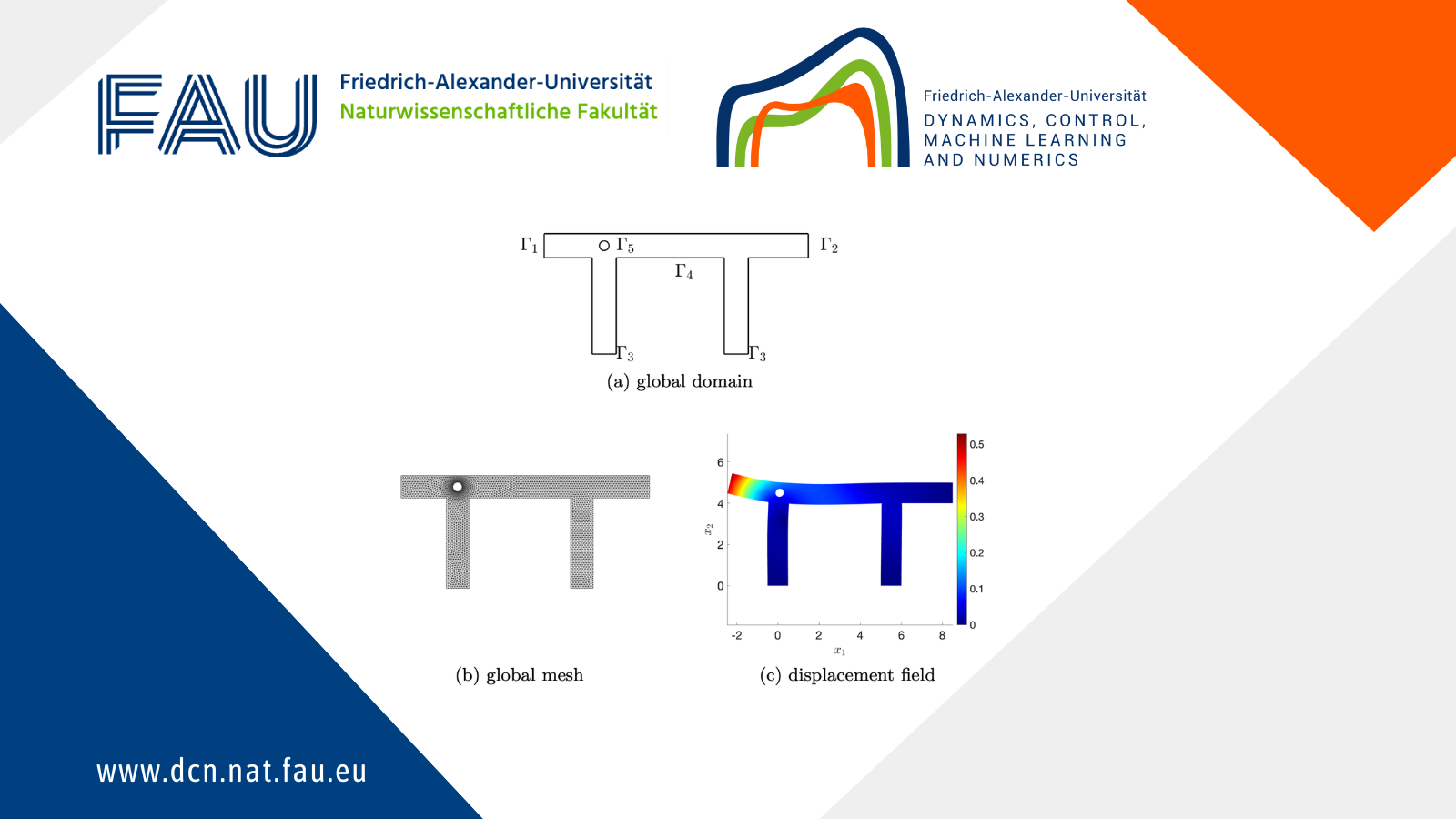
We investigate the performance of the proposed DD technique for a nonlinear elasticity study case. Let the domain \Omega \subset \mathbb{R}^2 be given and \partial \Omega= \Gamma_1 \cup \Gamma_2 \cup \Gamma_3 \cup \Gamma_4 \cup \Gamma_5 as in Figure 2(a).
Let \mathbf{n} denote the outward unit normal on \partial \Omega .
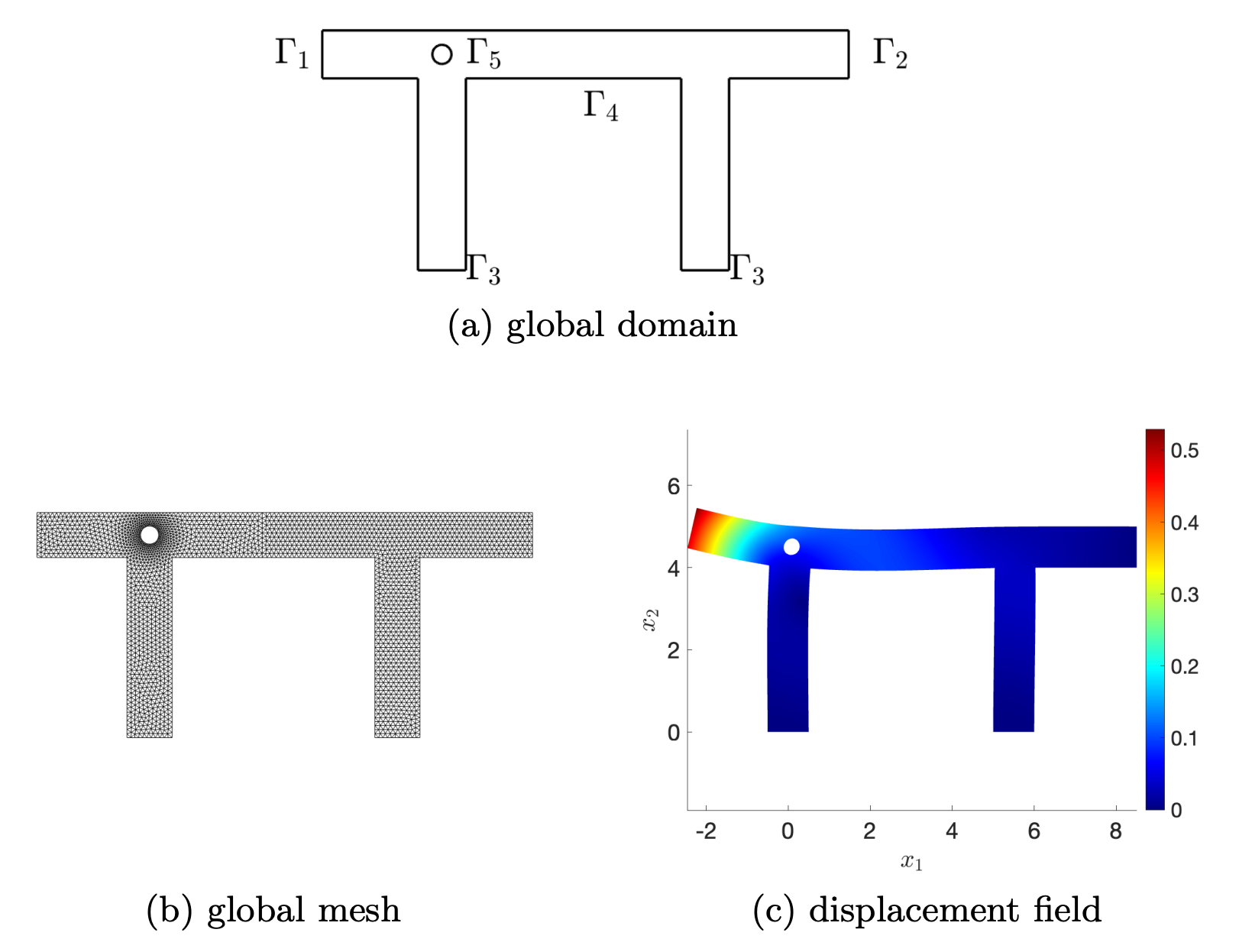
Figure 2. Global domain and solution \mathbf{u}_{\rm{glo}} to the global problem (1).
We consider the neo-Hookean model
\begin{cases} -\nabla \cdot \mathbf{P}(\mathbf{F}(\mathbf{u})) = 0 & \text{in } \Omega_{\text{glo}} \\ \mathbf{P}(\mathbf{F}(\mathbf{u})) \, \mathbf{n} = \mathbf{g}_{\text{neu}} = \begin{pmatrix} 1 \\ 0.25 \end{pmatrix} & \text{on } \Gamma_1 \\ \mathbf{u} = \mathbf{0} & \text{on } \Gamma_2 \cup \Gamma_3 \\ \mathbf{P}(\mathbf{F}(\mathbf{u})) \, \mathbf{n} = \mathbf{0} & \text{on } \Gamma_4 \cup \Gamma_5 \end{cases} \quad (1)
where \mathbf{F}(\mathbf{u}) = \mathbb{I} + \nabla \mathbf{u} is the deformation gradient and the stress is given by the first Piola-Kirchhoff stress tensor \mathbf{P} :
\mathbf{P}(\mathbf{F}) = \lambda_2 \mathbf{F} - \mathbf{F}^{-\top} + \lambda_1 \det(\mathbf{F}) \mathbf{F}^{-\top},
with the Lamé constants \lambda_1 and \lambda_2 defined in terms of the Young’s modulus E and Poisson’s ratio \nu as
\lambda_1 = \frac{E \nu}{(1 + \nu)(1 - 2\nu)},
\lambda_2 = \frac{E}{2(1 + \nu)}. We consider parameters \mu=0.33, E=100.
We depict in Figure 2(c) the solution displacement \mathbf{u}_{\rm{glo}}, obtained by Newton’s method with line-search.
We decompose the domain \Omega into two subdomains \Omega_{\rm{phys}} and \Omega_{\rm{data}} depicted in Figure 3.
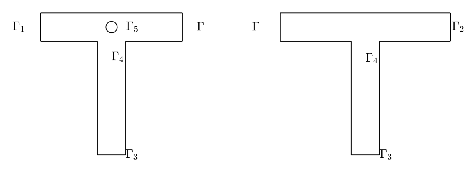
Figure 3. Geometric configurations of \Omega_{\rm{phys}} (left) and \Omega_{\rm{data}} (right).
3.2 Physics-data interface coupling
The PDIC solutions of Figure 4 have been obtained by gaussian process regression by using, in the training phase, n_{\rm{sample}}=90 random points at \Gamma.
The preliminary results show a good accuracy—with a relative error in the order of 1\%—also for the solution reconstructed at the interface \Gamma (cf. Table 1).
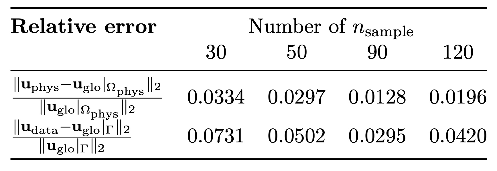
Table 1. Comparison of relative errors for different numbers of training points.
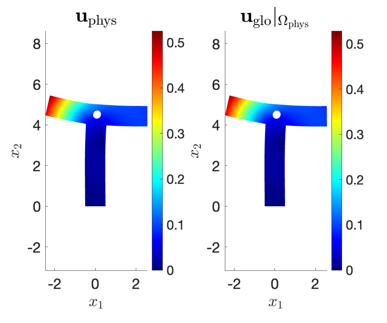
Figure 4. Comparison between (at left) the physical solution \mathbf{u}_{\rm{phys}} obtained in \Omega_{\rm{phys}} by the Physics Data Interface Coupling algorithm scheme and (at right) the global solution \mathbf{u}_{\rm{glo}}|_{\Omega_{\rm{phys}}}.
4 Conclusions
In this post, we introduced a flexible, general framework for solving multi-physics problems. As a first (multi-fidelity) test case, we applied it to a nonlinear elasticity problem — with promising results.
We’re currently adapting other domain decomposition methods, including the optimization-based algorithms (e.g., Taddei 2024), which treat interface fluxes as control variables. We’re also exploring the extension of the method to unsteady multi-physics problems.
References
[1] S. Deparis, M. Discacciati, A. Quarteroni (2006) A domain decomposition framework for fluid-structure interaction problems, Springer, Computational Fluid Dynamics 2004: Proceedings of the Third International Conference on Computational Fluid Dynamics, ICCFD3, pp.41-58[2] C. Wentland, R. Christopher, F. Rizzi, J. Barnett, I.K. Tezaur (2025) The role of interface boundary conditions and sampling strategies for Schwarz-based coupling of projection-based reduced order models, Elsevier, Journal of Computational and Applied Mathematics, Vol. 465, pp. 116-584
[3] T. Taddei, X. Xu, L. Zhang (2024) A non-overlapping optimization-based domain decomposition approach to component-based model reduction of incompressible flows, Journal of Computational Physics, Vol. 509, pp. 113-038
|| Go to the Math & Research main page

