
Using the support function for optimal shape design

1 Motivation
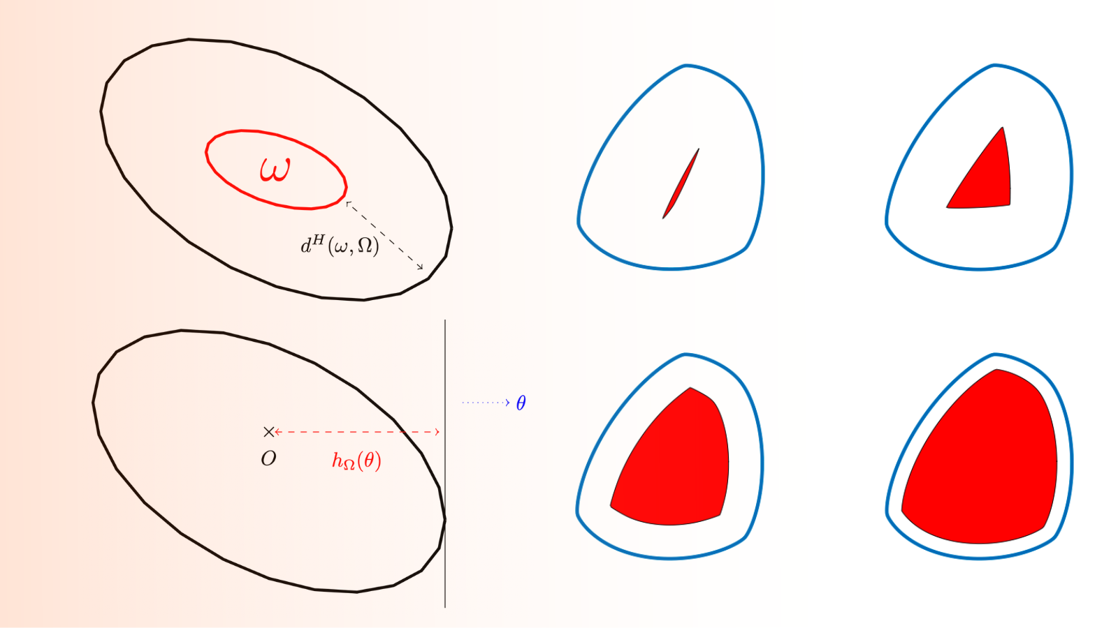
Led by problems of optimal placement and design of sensors, we are interested in considering the following shape optimization problem
\inf_{\omega\subset \Omega} d^H(\omega,\Omega), (1)
where d^H is the Hausdorff distance between \Omega and \omega defined as follows
d^H(\omega,\Omega):= \sup_{x\in \Omega} d(x,\omega),
with d(\cdot,\omega):= \inf_{y\in\omega}\|x-y\| is the distance from x to the set \omega.
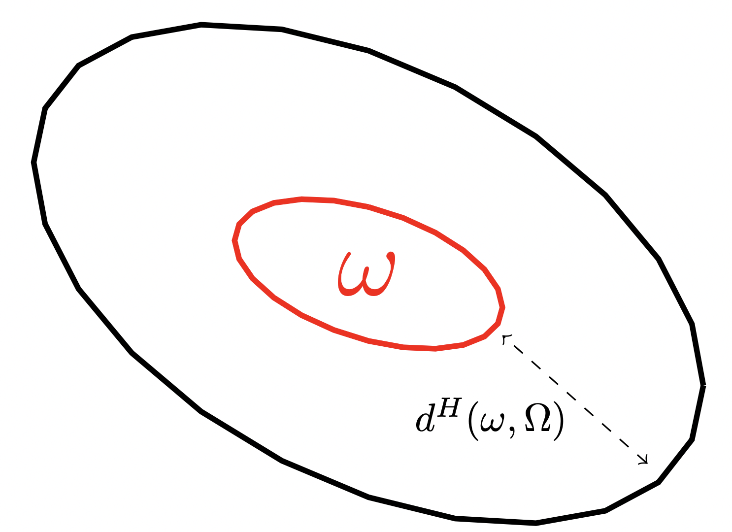
Figure 1. The Hausdorff distance between the sensor \omega and the set \Omega
If no additional assumption on the sensor is assumed, the problem (1) does not admit a solution. In this post, we ask the sensor to be convex, which provides existence of optimal shapes as shown in the following proposition:
Proposition 1.1
Let \Omega\subset \R^n be a bounded set. The problem
\inf\{ J_\Omega(\omega)\ |\ \omega\ \text{is convex,}\ \omega\subset \Omega\ \text{and}\ |\omega|=\alpha |\Omega|\},
with \alpha\in (0,1], admits a solution.
Proof
Let (\omega_n) be a minimizing sequence of convex sets, i.e., such that |\omega_n|= \alpha |\Omega| and
\lim_{n\rightarrow +\infty} d^H(\omega_n,\Omega) = \inf_{\underset{\omega\subset \Omega}{|\omega|=\alpha |\Omega|}} d^H(\omega,\Omega).
Since all the convex sets \omega_n are included in the bounded set \Omega, we have by Blaschke selection Theorem [???] that there exists a convex set \omega^*\subset \Omega such that (\omega_n) converges up to a subsequence (that we also denote by (\omega_n)) to \omega^* with respect to the Hausdorff distance. Finally, by the continuity of the area with respect to the Hausdorff distance, we have
\omega^*| = \lim_{n\rightarrow +\infty} |\omega_n| = \alpha |\Omega|,
which ends the proof.
In the present post, we assume the box \Omega to be convex and make use of the classical properties of convex sets to propose an algorithm which computes the optimal sensor.
1.1 Classical definitions and lemmas
If \Omega is convex (not necessarily containing the origin), its support function is defined as follows:
h_\Omega:x\in \R^2\longmapsto \sup\{\langle x,y \rangle\ |\ y\in \Omega\}.</p> <p style="text-align: center;">[katex] Since the functions [katex]h_\Omega satisfy the scaling property h_\Omega(t x) = t h_\Omega(x) for t>0, it can be characterized by its values on the unit sphere \mathbb{S}^{1} or equivalently on the interval [0,2\pi]. We then adopt the following definition:
Definition 1.2
The support function of a planar bounded convex set \Omega is defined on [0,2\pi] as follows:
h_\Omega:[0,2\pi)\longmapsto \sup\left\{\left\langle \binom{\cos{\theta}}{\sin{\theta}}, y \right\rangle\ |\ y\in\Omega\right\}.
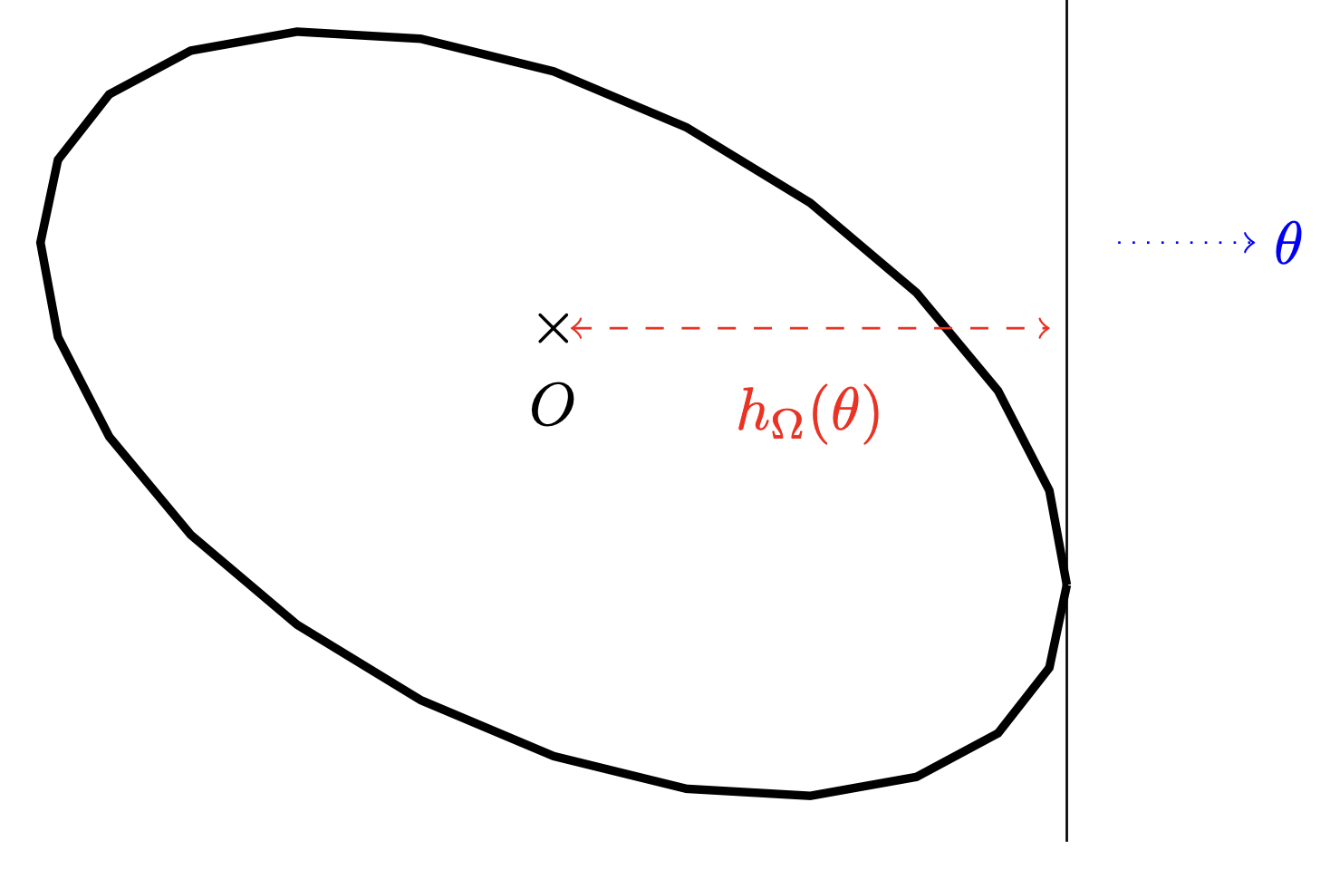
Figure 2. The Hausdorff distance between the sensor \omega and the set \Omega
The support function has some nice properties:
• It allows to provide a simple criterion of the convexity of \Omega. Indeed, \Omega is convex if and only if h_\Omega''+h_\Omega\ge 0 in the sense of distributions.
• It is linear for the Minkowski sum and dilatation. Indeed, if \Omega_1 and \Omega_2 are two convex bodies and \alpha, \beta >0, we have
h_{\alpha \Omega_1 + \beta \Omega_2}= \alpha h_{\Omega_1}+ \beta h_{\Omega_2},
see [2, Section 1.7.1].
• It allows to parametrize the inclusion in a simple way. Indeed, if \Omega_1 and \Omega_2 are two convex sets, we have
\Omega_1\subset \Omega_2\Longleftrightarrow h_{\Omega_1}\leq h_{\Omega_2}.
• It also provides elegant formulas for some geometrical quantities. Fro example the perimeter and the area of a convex body \Omega are given by
P(\Omega) = \int_0^{2\pi}h_\Omega(\theta)d\theta\ \ \ \text{and}\ \ \ |\Omega|= \frac{1}{2}\int_0^{2\pi} h_\Omega(\theta)(h_\Omega''(\theta)+h_\Omega(\theta))d\theta,
and the Hausdorff distance between two convex bodies \Omega_1 and \Omega_2 is given by
d^H(\Omega_1,\Omega_2)=\max_{\theta\in [0,2\pi]} |h_{\Omega_1}(\theta)-h_{\Omega_2}(\theta)|,
see [2, Lemma 1.8.14].
2 Description of the numerical method
2.1 Parametrization of the problem
We recall that if both \Omega and \omega are convex, we have the following characterization for the Hausdorff distance between \omega and \Omega,
d^H(\omega,\Omega)=\|h_\Omega-h_\omega\|_{\infty}:=\max_{\theta\in [0,2\pi]} |h_{\Omega_1}(\theta)-h_{\Omega_2}(\theta)|,
where h_\Omega and h_\omega respectively correspond to the support functions of the convex sets \Omega and \omega.
The use of the support function allows to transform the purely geometrical problem into the following analytical one:
\left\{\begin{matrix} \inf\limits_{h\in H^1_{\text{per}}(0,2\pi)} \|h_\Omega-h\|_{\infty},\\ h\leq h_\Omega,\\ h''+h\ge 0,\\ \frac{1}{2}\int_0^{2\pi} h(h''+h)d\theta = \alpha_0 |\Omega|. \end{matrix}\right. (2)
where H^1_{\text{per}}(0,2\pi) is the set of H^1 functions that are 2\pi-periodic.
In order to be able to perform numerical shape optimization, we have to retrieve a finite dimensional setting. The idea is to parametrize sets via Fourier coefficients of their support functions truncated at a certain order N\ge 1. Thus, we will look for solutions in the set
\mathcal{H}_N:= \left\{\theta\longmapsto a_0 + \sum_{k=1}^N \big(a_k \cos{(k\theta)}+ b_k\sin{(k\theta)}\big) \ \big|\ a_0,\dots,a_N,b_1,\dots,b_N\in \R\right\}.
This approach is justified by the following approximation proposition:
Proposition 2.1 ([2, Section 3.4])
Let \Omega\in \mathcal{K}^2 and \varepsilon>0. Then there exists N_\varepsilon and \Omega_\varepsilon with support function h_{\Omega_\varepsilon}\in \mathcal{H}_{N_\varepsilon} such that d^H(\Omega,\Omega_\varepsilon) \lt \varepsilon .
For more convergence results and application of this method for different problems, we refer to [1].
Thus, the infinitely dimensional problem (2) is approached by the following finitely dimensional problem.
\left\{\begin{matrix} \inf\limits_{(a_0,a_1,\dots,a_N,b_1,\dots,b_N)\in \R^{2N+1}} \max\limits_{\theta\in[0,2\pi]} h_\Omega(\theta) - a_0 - \sum\limits_{k=1}^N \big(a_k \cos{(k\theta)}+b_k\sin{(k\theta)}\big), \\ \forall \theta\in [0,2\pi], \ \ \ a_0+\sum\limits_{k=1}^N \big(a_k \cos{(k\theta)}+ b_k\sin{(k\theta)}\big)\leq h_\Omega(\theta), \\ \forall \theta\in [0,2\pi], \ \ \ h''+h\ge 0, \\ \frac{1}{2}\int_0^{2\pi} h(h''+h)= \alpha_0 |\Omega|. \end{matrix}\right.
Let M\in \N^*, we consider the regular subdivision (\theta_k)_{k\in \llbracket 1,M \rrbracket } of [0,2\pi], where \theta_k= \frac{2k\pi}{M}. The inclusion constraint h(\theta)\leq h_\Omega(\theta) and the convexity constraint h''(\theta)+h(\theta)\ge 0 are approximated by the following 2M linear constraints on the Fourier coefficients:
\forall k\in \llbracket1,M\rrbracket, \Bigg\{ \begin{array}{cc} a_0+\sum\limits_{j=1}^N \big(a_j \cos{(j\theta_k)}+ b_j\sin{(j\theta_k)}\big)\leq h_\Omega(\theta_k), \\ a_0+\sum\limits_{j=1}^N \big((1-j^2)\cos{(j\theta_k)}a_j + (1-j^2)\sin{(j\theta_k)}b_j \big) \ge 0. \end{array}
At last, straightforward computations show that the area constraint is equivalent to the following quadratic constraint:
\pi a_0^2 + \frac{\pi}{2} \sum\limits_{k=1}^N(1-k^2)(a_k^2+b_k^2)=\alpha_0 |\Omega|.
2.2 Computation of the gradients
A very important step in shape optimization is the computation of the gradients. In our case, the convexity and inclusion constraints are linear and the area constraint is quadratic (and thus its gradient is obtained by direct computations). Nevertheless, the computation of the gradient of the objective function is not straightforward as it is defined as a supremum. This is why we use a Danskin differentiation scheme to compute the derivative.
Proposition 2.2
Let us consider
g:(\theta,a_0,\dots,b_N)\longmapsto h_\Omega(\theta) - a_0 - \sum\limits_{k=1}^N \big(a_k \cos{(k\theta)}+b_k\sin{(k\theta)}\big)
and
j:(a_0,\dots,b_N)\longmapsto \max_{\theta \in [0,2\pi]} g(\theta,a_0,\dots,b_N).
The function j admits directional derivatives in every direction and we have
\frac{\partial j}{\partial a_0} = -1,
and for every k\in\llbracket 1,N \rrbracket,
\left\{\begin{matrix} \frac{\partial j}{\partial a_k} = \max\limits_{\theta^*\in \Theta} -\cos{(k \theta^*)}, \\ \frac{\partial j}{\partial b_k} = \max\limits_{\theta^*\in \Theta} -\sin{(k\theta^*)}, \end{matrix}\right.
where
\Theta:=\{\theta^*\in [0,2\pi]\ \ |\ \ G(\theta^*,a_0,\dots,b_N) = \max\limits_{\theta\in[0,2\pi]} G(\theta,a_0,\dots,b_N)\}.
Proof
Since the same scheme is followed for every coordinate, we limit our selves to present the proof for the fist coordinate a_0. In order to simplify the notations, we will write for every x\in \R, j(x) = j(a_0,\dots,a_{k-1},x,a_{k+1}\dots,b_N) and G(\theta,x) = G(\theta,a_0,\dots,a_{k-1},x,a_{k+1}\dots,b_N).
For every t\ge0, we denote by \theta_t\in[0,2\pi] a point such that
G(\theta_t,a_k+t) = j(a_k+t) = \max\limits_{\theta\in [0,2\pi]} G(\theta,a_k+t).
We have
j(a_k+t)-j(a_k)= G(\theta_t,a_k+t)-G(\theta_0,a_k) \ge G(\theta_0,a_k+t)-G(\theta_0,a_k)= -t \cos{(k \theta_0)}.
Thus,
\forall \theta_0\in \Theta,\ \ \ \liminf_{t\rightarrow 0^+} \frac{j(a_k+t)-j(a_k)}{t} \ge -\cos{(k \theta_0)},
which means that
\liminf_{t\rightarrow 0^+} \frac{j(a_k+t)-j(a_k)}{t} \ge \max\limits_{\theta_0\in \Theta}-\cos{(k \theta_0)}. (3)
Let us now consider a sequence (t_n) of positive numbers decreasing to 0, such that
\lim_{n\rightarrow +\infty} \frac{j(a_k+t_n)-j(a_k)}{t_n} = \limsup_{t\rightarrow 0^+} \frac{j(a_k+t)-j(a_k)}{t}.
We have for every n\ge 0,
j(a_k+t_n)-j(a_k)= G(\theta_{t_n},a_k+t_n)-G(\theta_0,a_k)\leq G(\theta_{t_n},a_k+t_n)-G(\theta_{t_n},a_k)=-t_n\cos{(k \theta_{t_n})}.
Thus,
\limsup_{t\rightarrow 0^+} \frac{j(a_k+t)-j(a_k)}{t} = \lim_{n\rightarrow +\infty} \frac{j(a_k+t_n)-j(a_k)}{t_n} \leq \limsup_{n\rightarrow +\infty}-\cos{(k\theta_{n})}=-\cos{(k\theta_{\infty})},
where \theta_\infty is an accumulation point of the sequence (\theta_n). It is not difficult to check that \theta_\infty \in \Theta. Thus, we have
\limsup_{t\rightarrow 0^+} \frac{j(a_k+t)-j(a_k)}{t} \leq \max\limits_{\theta_0\in \Theta}-\cos{(k \theta_0)}. (4)
By the inequalities (3) and (4) we deduce the announced formula for the derivative.
2.3 Numerical results
Now that we have parameterized the problem and computed the gradients, we are in position to perform shape optimization. We use the 'fmincon' Matlab routine. We consider a smooth set whose support function is given by
h_\Omega(t) = 9 + 0.1 \cos{t}-0.3\cos{2t} +0.2\cos{3t}-0.03\cos{4t}-0.1\cos{5t}+0.1\sin{t}-0.2\sin{2t} +0.1\sin{3t}-0.01\sin{4t}-0.01\sin{5t}.
and the area proportion \alpha_0\in \{0.01,0.1,0.4,0.7\}.
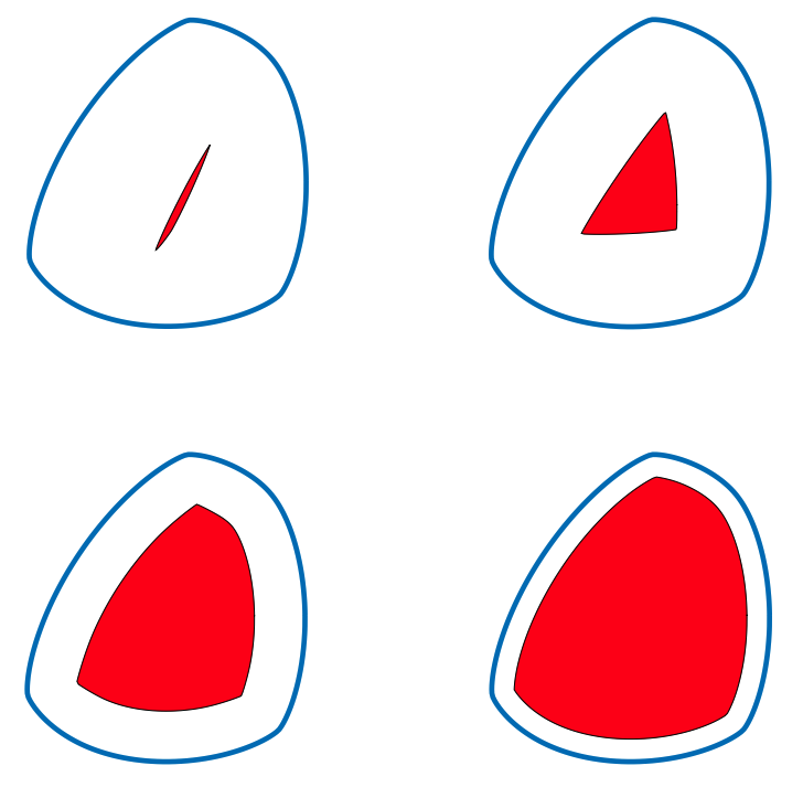
Figure 3. The optimal shape for \alpha_0\in \{0.01,0.1,0.4,0.7\}.
References
[1] P. R. S. Antunes and B. Bogosel. Parametric shape optimization using the support function. Comput. Optim. Appl., 82(1):107–138, 2022.[2] R. Schneider. Convex Bodies: The Brunn-Minkowski Theory. Cambridge University Press, 2nd expanded edition edition, 2013.
|| Go to the Math & Research main page


