

Boundary and Interior Control in a Diffusive Lotka-volterra Model
 João Carlos Fernandes Barreira
1 Introduction
1.1 Problem formulation and main results
In this post, we consider a general diffusive Lotka-Volterra Model (LVM) for two competing species. The system, with boundary controls and an interior multiplicative control, is described by
\left\{\begin{array}{ll} u_t=d_1\Delta u+u(a_1-b_1u-c_1v)+h1_{\omega}u,& (x,t)\in\Omega\times\mathbb{R}^+\\ v_t=d_2\Delta v+v(a_2-b_2u-c_2v),& (x,t)\in\Omega\times\mathbb{R}^+\\ (u(x,0),v(x,0))=(u_0,v_0),& x\in\Omega\\ u(x,t)=c_u(x,t),\ \ v(x,t)=c_v(x,t),& (x,t)\in\partial\Omega\times\mathbb{R}^+, \end{array} \right. (1)
where a_i, b_i, c_i, d_i ( i = 1, 2) are positive parameters, and \Omega \subset \mathbb{R}^N ( N = 1, 2, 3 ) is a smooth domain with a regular boundary \partial\Omega. The term h 1_{\omega} u represents an interior multiplicative control, where \omega \subset \Omega is a non-empty open set, 1_{\omega} is the characteristic function of \omega, and c_u, c_v are boundary controls.
For the uncontrolled system, the carrying capacities of u and v are a_1/b_1 and a_2/c_2 , respectively. Therefore, it is natural to impose constraints on the solutions based on these values, i.e.,
0\leq u\leq a_1/b_1,\ \ 0\leq v\leq a_2/c_2. \hspace{1cm}(2)
Similarly, we have the following constraints on the boundary controls:
0\leq c_u\leq a_1/b_1,\ \ 0\leq c_v\leq a_2/c_2. \hspace{1cm}(3)
On the one hand, conditions (2) and (3) increase the complexity of the problem, but on the other hand, they bring it closer to the conditions of physical reality and are one of the key aspects that make the problem more challenging and significant.
Initially, we consider the following target (0, a_2/c_2) , a steady state of (1) which represents the survival of one species (v) at its carrying capacity, and the extinction of the other (u). For this case, the following theorem guarantees the existence of controls on the boundary and within the domain, all depending solely on the spatial variable, which asymptotically guide the trajectories towards this target.
Theorem 1
Suppose \omega=\Omega, then there are boundary controls c_u, c_v\in L^{\infty}(\partial\Omega) and an interior control h\in L^{\infty}(\Omega) such that, for every (u_0,v_0)\in L^{\infty}(\Omega)\times L^{\infty}(\Omega), the solution (u,v) of (1) satisfies
\lim_{t\to\infty}(u(\cdot, t),v(\cdot,t))=(0,a_2/c_2)
uniformly in \Omega.
For the proof, the controls (c_u(x), c_v(x)) = (0, a_2/c_2) are defined on the boundary of the region \partial \Omega , and, for simplicity, h(x) = \sigma within the region \Omega , where \sigma is a constant that satisfies the following condition:
-a_1 \lt \sigma \lt \lambda_1d_1-a_1.
Next, a stationary solution (u^s, v^s) is considered for the stationary system associated with (1), where c_u , c_v , and h are defined as mentioned above. Through a multiplication and integration analysis, it is concluded that u^s \equiv 0 . From this, it follows that v^s \equiv a_2/c_2 . Therefore, the stationary state is unique and given by (0, a_2/c_2) .
Additionally, based on the main result from [2], any bounded solution of the system will converge to this stationary state. That is, we have
\lim_{t \to \infty} (u(x,t), v(x,t)) = (0, a_2/c_2)
uniformly in \Omega , where (u,v) is the solution of (1) with \omega = \Omega and the controls provided by as in the beginning.
By symmetry, we then obtain an analogous result to Theorem 1 for the target \left( {a_1}/{b_1}, 0 \right) , when the internal control acts exclusively on the second equation of the system.
Therefore, for the targets (a_1/b_1,0) and (0,a_2/c_2), we establish a global asymptotic controllability result. That is, given any initial condition satisfying the constraints (2), we construct boundary controls c_u and c_v, along with a bounded interior control h (assuming \omega = \Omega in this case), that steer the trajectories toward the target as t \to \infty. As discussed by [3], when considering only boundary controls in a particular weak competition model (that is, when in our model (1) we consider c_1,b_2 \lt 1, a_{1}=1, b_1=1, and c_2=1), if b_2 \lt a_2 \lt 1/c_1 and \lambda_1 \lt \min\lbrace (1-a_2c_1)/d_1,(a_2-b_2)/d_2 \rbrace then a barrier effect arises. This means that barriers can be designed to prevent trajectories from reaching the desired targets, regardless of the boundary controls, which may vary in space and time. In this context, internal control plays a crucial role. The multiplicative control, acting as a potential, enables trajectories to overcome potential barriers and gradually steer toward the target.
The second target concerns a case of heterogeneous coexistence within the specific scenario d_1 = d_2 = d , a_1 = a_2 = a ,
(u^{**}(x),v^{**}(x))=\left(\left(\dfrac{c_2-c_1}{b_1c_2-c_1b_2}\right)\theta,\left(\dfrac{b_1-b_2}{b_1c_2-c_1b_2}\right)\theta\right) \hspace{1cm}(4)
where \theta=\theta(x) is a smooth function that satisfies
\left\{\begin{array}{l} d\Delta\theta+\theta(a- \theta)=0,\ \ x\in \Omega \\ \theta=0,\ \ x\in\partial\Omega\\ 0 \lt \theta \lt 1,\ \ x\in \Omega. \end{array}\right. \hspace{1cm}(5)
In this case, we also assume b_1 > b_2 , c_1 \lt c_2 to ensure the positivity of u^{**} and v^{**} in \Omega.
Before stating our next theorem, we need to consider the following eigenvalue problem
\left\{\begin{array}{ll} \Delta\phi+\lambda\phi=0,& x\in\Omega\\ \phi=0,& x\in\partial\Omega. \end{array}\right. \hspace{1cm}(6)
We denote by \lambda_1 the smallest eigenvalue of (6), and it is well known that \lambda_1 > 0.
Thus, we are able to state our second result.
Theorem 2
Assume that d_1=d_2=d, a_1=a_2=a, b_1>b_2, c_1 \lt c_2, and let any nonempty open set \omega\subset\Omega. If
d \lt \dfrac{a}{\lambda_1} \hspace{1cm}(7)
then for every (u_0,v_0)\in L^{\infty}(\Omega)\times L^{\infty}(\Omega) there are boundary controls c_u, c_v\in L^{\infty}(\partial\Omega) and an interior control h\in L^{\infty}(\omega\times (0,T)), such that the solution associated (u,v) of (1) satisfies
(u(\cdot, T),v(\cdot,T))=(u^{**},v^{**}), \hspace{1cm}(8)
for some T>0.
The proof is performed in two steps: in the first step, we will show that, under specific conditions on the parameters and considering the internal control identically null, the asymptotic control result for the target (u^{**}, v^{**}) is achieved; in the second step, the result concerning local null control will be established through the Inverse Mapping Theorem (see, [1]).
Therefore, Theorem 2 states that the target (u^{**},v^{**}) can be exactly reached in finite time when (7) holds. This inequality, which relates the geometry of the domain \Omega (represented by \lambda_1), the diffusion capacity, and the reproduction rate of the species, is necessary for the asymptotic approximation to the target, which corresponds to the first step of the control strategy.
The finite-time controllability obtained in Theorem 2 is particularly interesting because, although we have 0 \lt u^{**}(x) \lt a_1/b_1 and 0 \lt v^{**}(x) \lt a_2/c_2 for x \in \Omega, we also have u^{**}(x) = v^{**}(x) = 0 for x \in \partial\Omega. As a consequence, the trajectory oscillations generally required to achieve finite-time controllability could potentially violate some of the constraints, given that the target vanishes at the boundary. However, we establish a strategy that prevents this issue. This is made possible primarily due to the adopted multiplicative interior control. Indeed, the idea is that, given any initial condition satisfying (2), we keep the interior control h \equiv 0 as well as the boundary controls c_u \equiv c_v \equiv 0. Under these conditions, the system’s dynamics drive the trajectories asymptotically toward the target. Then, once they are sufficiently close, we activate h and establish a finite-time local controllability result to ensure that the target is reached exactly (see Figure \ref{des}).
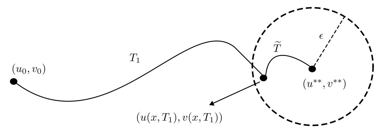
Figure 1. Controlled trajectory reaching exactly the target (u^{**},v^{**}) at time T=T_1+\widetilde{T}.
It is immediate that, under the same hypotheses of Theorem 2, we obtain the existence of boundary controls c_u, c_v \in L^{\infty}(\partial\Omega) and an interior control \bar{h} \in L^{\infty}(\omega \times (0,T)) (acting on the second equation) such that the associated solution (u,v) satisfies the (8).
Biological understanding and control
Biologically, the interior multiplicative control h1_{\omega} u acts as an external agent directly affecting the reproduction rate of u within a subregion \omega of the environment. The diffusive effect of the model spreads the influence of the control throughout the rest of the domain. Where h is positive, it may represent, for instance, a resource supplement that enhances the survival of u, or a genetic or environmental factor that increases the population growth rate of u. Conversely, where h is negative, the growth rate of u is reduced, which may result from a pesticide or a disease affecting only u. It is important to emphasize that, due to the biological interpretation of the model proposed here, in addition to the constraints on the boundary controls and the states, we must ensure that h remains bounded. In fact, control problems typically guarantee an L^2 regularity for the control, which is not sufficient for our purposes. Therefore, the L^{\infty} estimates obtained here for h are essential, and the arguments employed can be generalized and may be of independent interest.
The coupling between the equations ensures that an interior control acting solely in the first equation also affects, albeit indirectly, the species whose evolution is described by the second equation. Symbolically, h\sim u\sim v.
The boundary controls c_u and c_v directly influence the population densities of u and v at the boundary of the habitat, respectively. In this sense, these controls can have various interpretations. For instance, they may represent the forced relocation of individuals at the habitat boundaries, as in a population management program, or even a biological control strategy through the introduction of predators or the removal of competitors at the boundary.
It is worth emphasizing that, while this work focuses on Dirichlet controls, the same findings can be extended to Neumann controls. In particular, once Dirichlet controls that guide the solution toward the desired target are determined, the corresponding boundary flux can naturally be regarded as a Neumann control. This interplay is inherent in problems where controls are applied along the entire boundary. Hence, the results presented here can also be interpreted as strategies for regulating boundary flux, with practical implications in areas such as boundary regulation, filtration, and migration facilitation.
Numerical Simulations
As we have seen, the dynamics of the problem considered here guarantees us an asymptotic approximation to the targets (0,a_2/c_2) and (a_1/b_1,0), using a combination of boundary controls and a bounded multiplicative control in
the interior.
We simulate the effect of the multiplicative control h in driving the trajectories across barrier functions for the targets (0,a_2/c_2) and (a_1/b_1,0) . For the target (u^{**}, v^{**}) , the boundary controls guide the trajectories close to the target, while the internal multiplicative control h ensures that the trajectory reaches the target exactly at time T . In this case, we simulate the optimal control with respect to the minimum time and compare the results with and without activating h .
In addition to visualizing the behavior of the trajectories and controls, our goal is also to observe that, as expected, the internal control h can also contribute to the speed at which the trajectories can approaches the target.
The simulations were conducted using the software Matlab and the package Casadi.
For simplification and better understanding of the simulations, we chose a one-dimensional domain \Omega=(0,L)\subset\mathbb{R}. In this case, it is possible to explicitly determine the value of \lambda_1 in the estimate (7), namely, \lambda_1=\pi^2/L^2.
Crossing Barriers
Here, we consider the following parameter values: c_1 = 0.8, c_2 = 0.7, a_1 = a_2 = b_1 = b_2 = 1, d_1 = d_2 = 0.1, and L = 10. In this case, it is possible to prove that a barrier exists for the target (a_1/b_1,0)=(1,0) if no internal control is applied. The barrier is a nontrivial solution of
\left\{\begin{array}{ll} d_1\Delta u+u(1-u-c_1v)=0,& x\in \Omega,\\ d_2\Delta v+v(a_2-v-b_2u)=0,& x\in \Omega,\\ u(x)=1,\ \ v(x)=0,& x\in\partial\Omega, \end{array}\right. \hspace{1cm}(9)
and its existence was proven in [3].
Figure 2 shows the barriers (black dashed lines) preventing the trajectories from approaching the target. Note that, in this case, we set the boundary values as c_u=1 and c_v=0, and the same would hold for any other values satisfying the assumed constraints.
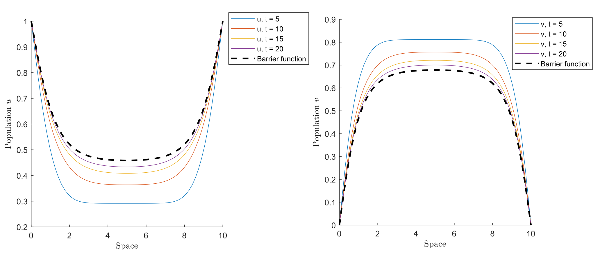
Figure 2. Barriers preventing the trajectories from approaching the target (a_1/b_1,0)=(1,0).
By activating a multiplicative control in the interior of the domain, we can see in Figure 3 the trajectories crossing the barrier and approaching the target (1,0). In this case, the control acted in the equation for v and in this simulation, we set {h}=-0.8.
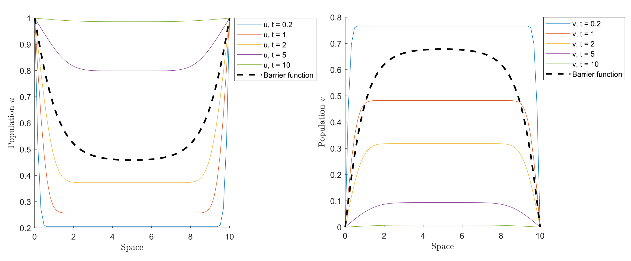
Figure 3. Trajectories crossing the barrier under the action of the internal control \overline{h}.
Optimal Control – Minimum Time
In what follows, we present simulations involving the target (u^{**},v^{**}) (see \eqref{uev}). Here, we assume
d_1 = d_2=d=1,
a_1 = a_2=a= 10, b_1 = 1.8, c_1 = 0.2,
b_2 = 1, c_2 = 1.4 and L=1.
Moreover, we assume the initial condition (u_0,v_0)=(0.2,0.3) and, to simplify the simulation, we considered \omega = (0,L) = (0,1) . Under these assumptions, inequality (7) is satisfied as well as the other conditions of Theorem 2. With the parameters adopted above, the target (u^{**},v^{**}) can be observed in Figure 4.
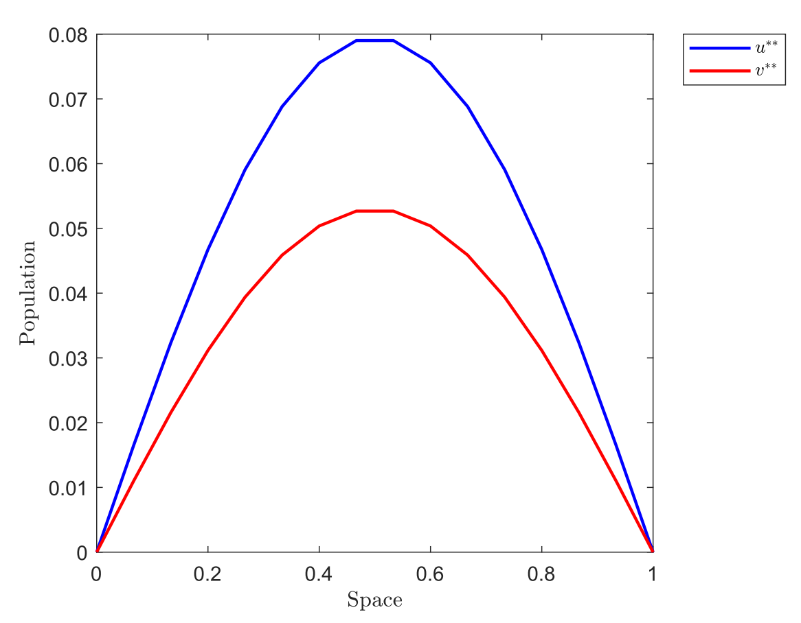
Figure 4. The target (u^{**},v^{**}).
We are interested in the controls c_u, c_v, and h that drive the trajectory to reach the target (with a tolerance of 10^{-2}) starting from the initial condition (u_0, v_0) = (0.2, 0.3). We recall that constraints must be assumed on the controls c_u and c_v (see (3)), and h must be bounded. In our example, we again assume |h| \leq 1. The minimum time obtained was t = 1.8055, and Figures 5 and 6 display the behaviors of u and v, respectively.
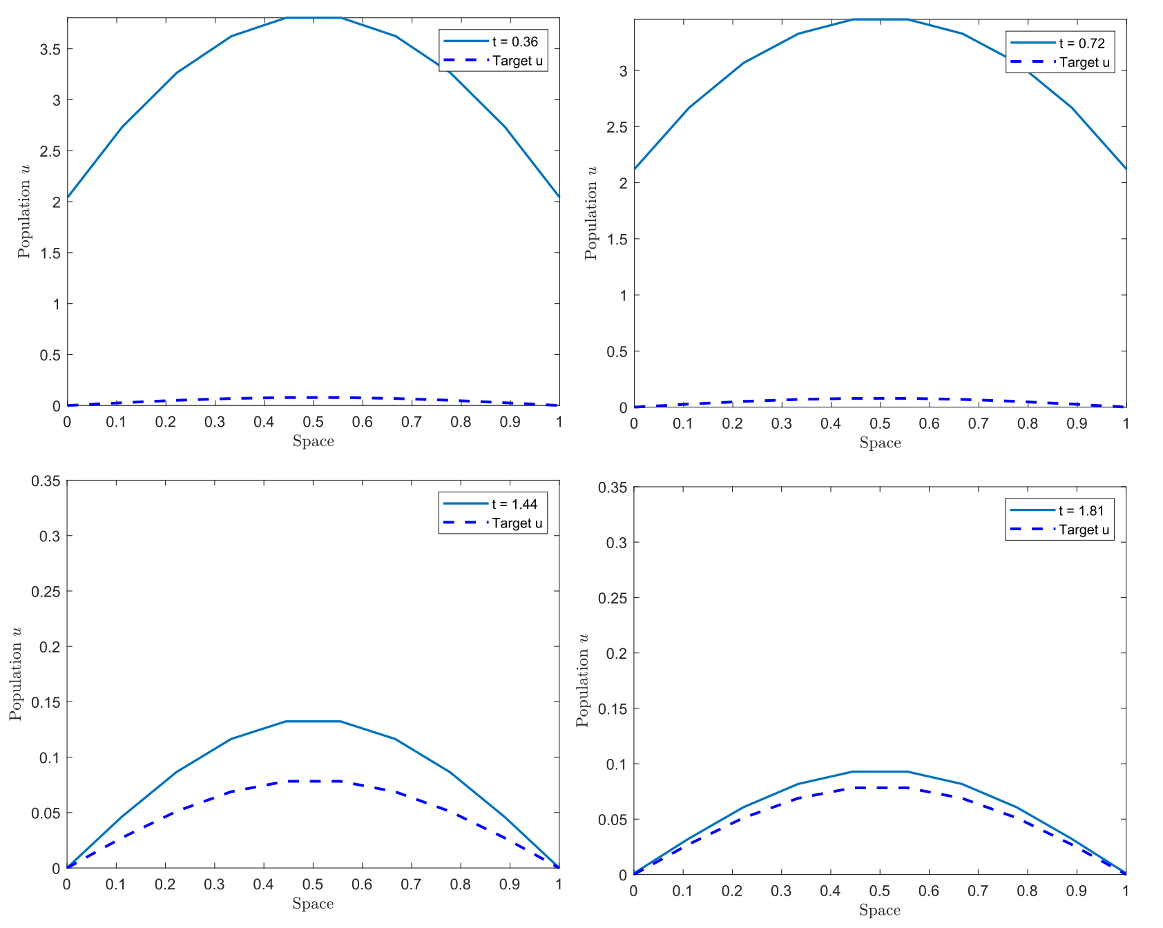
Figure 5. Trajectories approaching u^{**}.
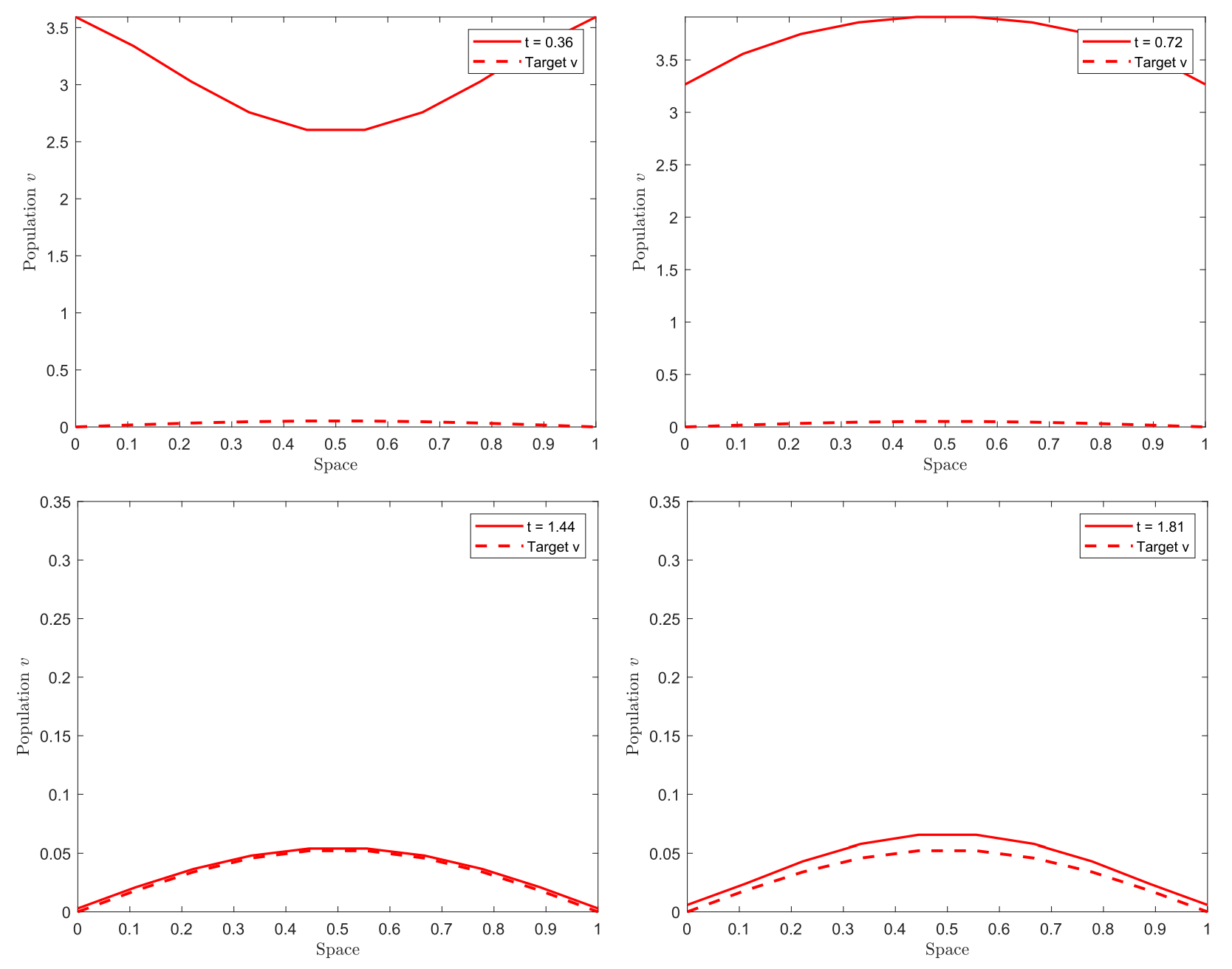
Figure 6. Trajectories approaching v^{**}.
The behavior of the controls c_u, c_v, and h can be observed in Figures 7 and 8, respectively.
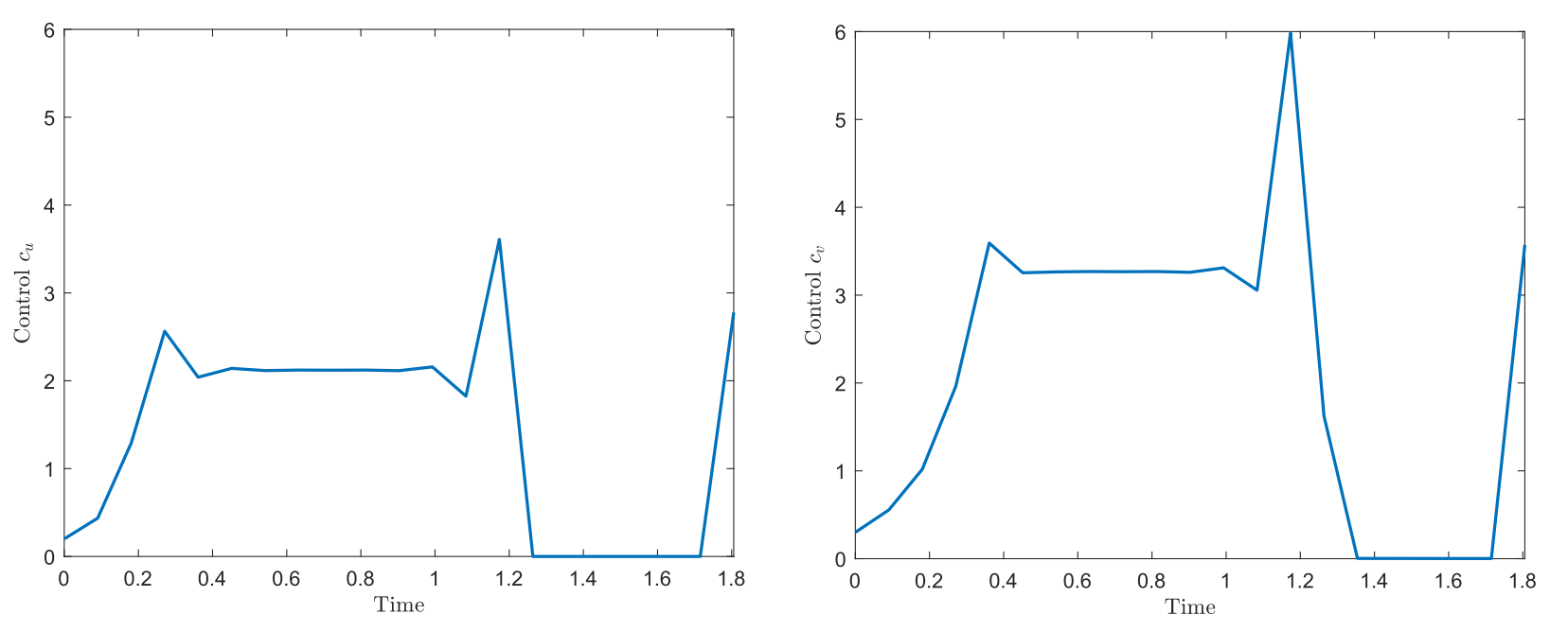
Figure 7. Boundary controls c_u and c_v.
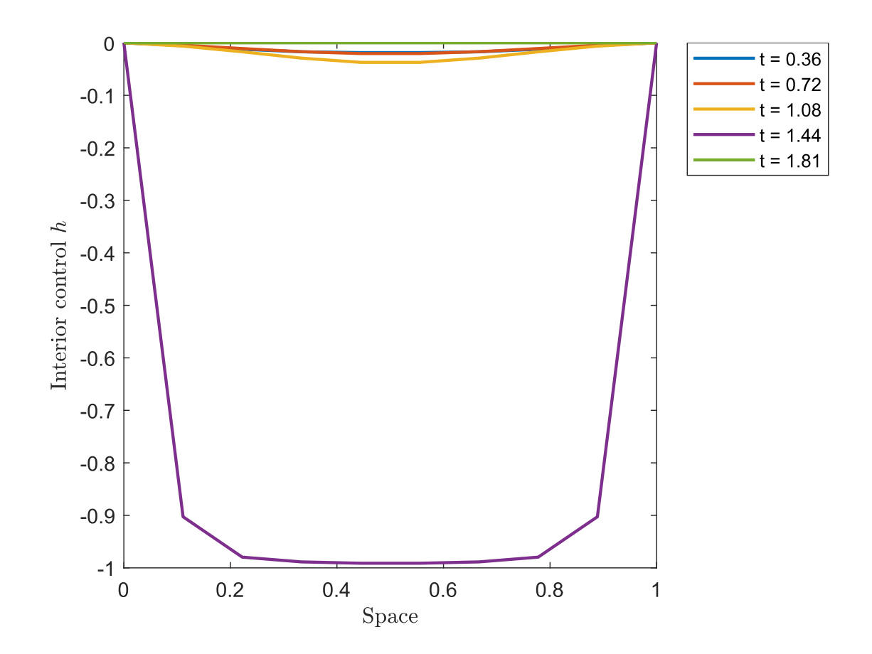
Figure 8. Interior control h.
In this case, we observe an interesting interplay between the boundary controls and the interior control in achieving the target in minimum time. Since the initial condition is above the desired target, h remains negative, reaching its lowest value at t = 1.44 before approaching zero as the trajectory nears the target. Meanwhile, c_u and c_v exhibit similar behavior on different scales, likely influenced by the initial conditions.
It is interesting to observe the initial behavior of the trajectories, which seems unrelated to the objective of approaching the target.
This reflects a dynamic rebalancing that the controls must achieve to drive the trajectory to a target that is positive in the interior of the domain and zero at the boundary.
The simulation of the same problem, but without considering the internal control h, results in a minimum time of t=2.0083. This shows that, in addition to allowing the target to be reached in finite time, the internal control accelerates the approach. The trajectories of u and v, as well as the controls c_u and c_v, can be seen in Figures 9 and 10, respectively.
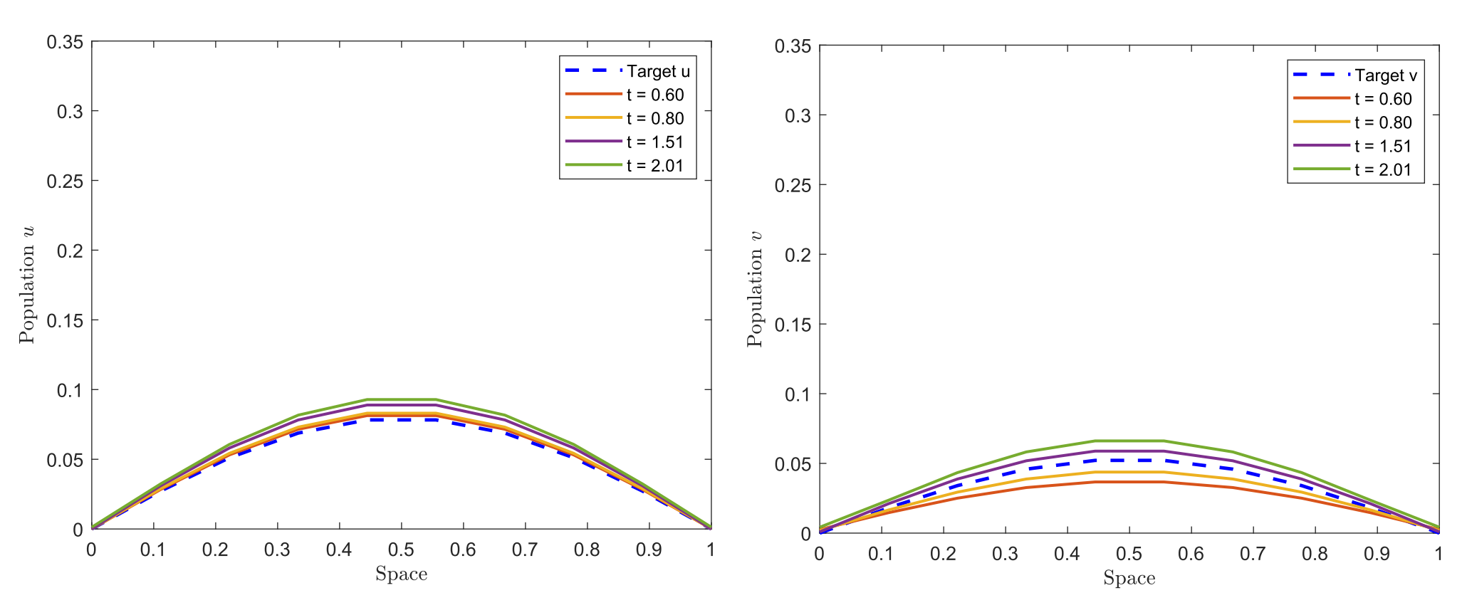
Figure 9. Trajectories of u and v without interior control.
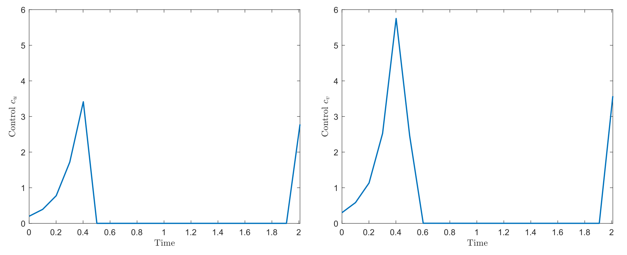
Figure 10. Boundary controls c_u and c_v without interior control.
In this case, we observe the trajectories and the controls on the boundary c_u and c_v in a more natural manner; however, as expected, with a minimum time greater than in the previous case.
Conclusion
We analyze the global controllability of a Lotka-Volterra model describing the competition between two species in a smooth domain \Omega \subset \mathbb{R}^N (N=1,2,3). The results are obtained by combining constrained boundary controls with a bounded multiplicative internal control. Below, we provide a comprehensive analysis of the results for each considered target.
• Survival of one of the species: (a_1/b_1,0) and (0,a_2/c_2).
This case is addressed in Theorem 1, and the asymptotic controllability is achieved through the combination of controls acting on the boundary and in the interior. More specifically, we provide boundary controls c_u and c_v satisfying (3), along with a multiplicative interior control hu such that for any initial condition (u_0, v_0) (0 \leq u_0 \leq a_1/b_1 and 0 \leq v_0 \leq a_2/c_2), The trajectory converges to the desired target as t\to\infty. This result holds independently of the problem parameters and the domain \Omega . As mentioned earlier, achieving finite-time controllability for these targets is particularly challenging due to the considered constraints on controls and trajectories.
• Heterogeneous coexistence: (u^{**},v^{**}).
In this case, Theorem 2 provides finite-time global controllability; roughly speaking, the target is exactly reached at some time T from any initial condition satisfying the constraints. This case is particularly interesting since the target (u^{**}, v^{**}) is zero on the boundary, and thus finite-time controllability could require some oscillation of the trajectories, potentially leading to a violation of one of the constraints. However, the interior multiplicative control h1_{\omega}u , combined with an appropriate control strategy, allows us to consider h sufficiently small so that comparison arguments can be used to ensure the assumed constraints.
References
[1] V.M. Alekseev, V.M. Tikhomorov, S. Formin (1987) Optimal control. Contemporary Soviet Mathematics. New York: Consultants Bureau[2] J. Smillie (1984) Competitive and cooperative tridiagonal systems of differential equations. SIAM Journal on Mathematical Analysis, Vol. 15, No. 3, pp.530-534.
[3] M. Sonego, E. Zuazua (2025) Control of a Lotka-Volterra system with weak competition.
|| Go to the Math & Research main page


