Clustering in discrete-time self-attention

Since the article Attention Is All You Need [1] published in 2017, many Deep Learning models adopt the architecture of Transformers, especially for Natural Language Processing and sequence modeling. These Transformers are essentially composed of layers, alternating between self-attention layers and feed forward layers, with normalization in-between.

In this post, we will explain the idea behind self-attention, and establish results on the behavior of a model composed only of self-attention layers with normalization.

1 What is self-attention?

When trying to analyze a sentence – whether to classify it, complete it, translate it, etc. – it is necessary to understand the relations between the words.

In order to do so, a first step is to turn each word into a vector, of dimension denoted by $d$ . This step, called “embedding”, can be accomplished by simply storing a dictionary which associates a vector to each word.

Once this is done, we then have $n$ vectors $x_1, \dots, x_n$ where $n$ is the number of words in the sentence.

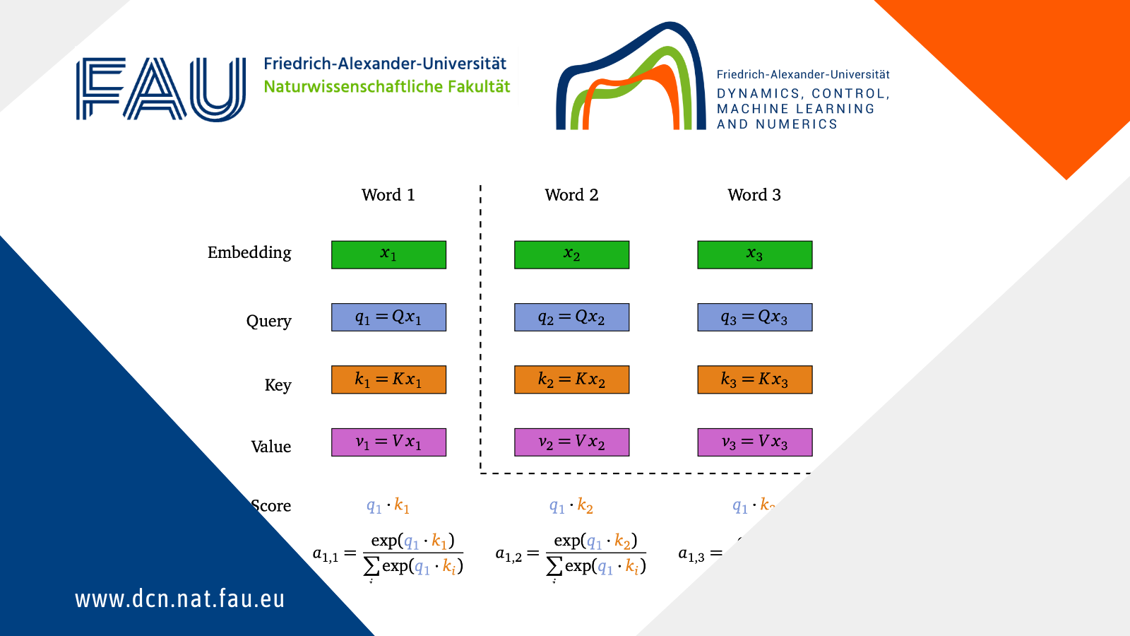
Let us focus on $x_1$ . To understand its relation with the different words in the sentence, an idea would be to look at the dot products $\langle x_1, x_i \rangle$ for $i \in [n]$ . However, we cannot really expect this dot product to really reflect the link between $x_1$ and $x_i$ . To have better chances at understanding this relation, we instead consider $\langle Qx_1, Kx_i \rangle$ for two matrices $Q, K \in \R^{d\times d}$ that will be learnt during training ( $Q$ stands for “Query”, and $K$ for “Key”). Then, the idea is that the larger $\langle Qx_1, Kx_i \rangle$ is, the more word $i$ is important in order to understand word $1$ . And we can turn these numbers into a probability distribution by setting

$a_{1, i} := \dfrac{\exp(\langle Qx_1, Kx_i \rangle)}{\sum\limits_{j = 1}^n \exp(\langle Qx_1, Kx_j \rangle)}.$

The idea is that the self-attention layer we are building will return, instead of $x_1$ , a vector that relies on these coefficients $a_{i, j}$ . More precisely, given a matrix $V\in\R^{d\times d}$ (where $V$ stands for “Value”), it will return $\sum\limits_{i = 1}^n a_{1, i} Vx_i$ (see, e.g. Figure 1).

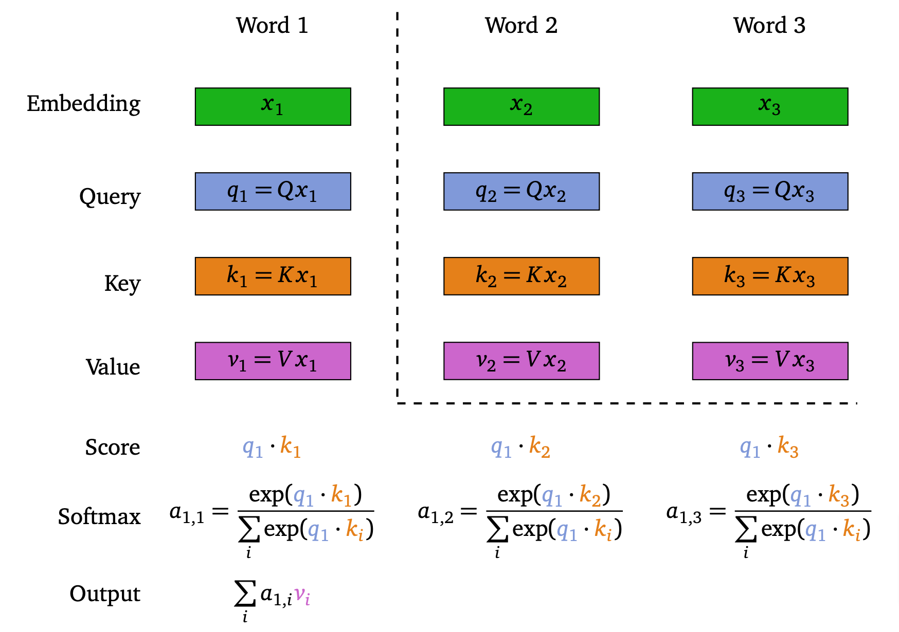
Figure 1. Illustration of a self-attention layer, for the first word as query

And the self-attention layer does this for each of the words in the sentence, after which each of the obtained vectors is normalized.

So, when stacking several self-attention layers, if $x_k^{(i)}$ is the $i^{\text{th}}$ vector after layer $k$ , we have

$\left\{ \begin{array}{ll} y_{k+1}^{(i)} & = x_k^{(i)} + \displaystyle\sum_{j = 1}^n \frac{e^{\beta \langle Q_k x_k^{(i)}, K_k x_k^{(j)} \rangle}}{Z_{\beta, i}(k)} V_k x_k^{(j)} \\ x_{k + 1}^{(i)} & = \displaystyle\frac{y_{k+1}^{(i)}}{\| y_{k+1}^{(i)} \|}, \end{array} \right.$

where $Z_{\beta, i}(k) := \sum\limits_{j = 1}^n e^{\beta \langle Q_k x_k^{(i)}, K_k x_k^{(j)} \rangle}$

, and $Q_k, K_k, V_k \in \R^{d\times d}$ .

As explained before, in practice, we would use a neural network between two self-attention layers, but in this post, we discard them.

2. Convergence result

The idea behind matrices $Q$ and $K$ is that the dot product $\langle x_i, x_j \rangle$ has no reason to really measure the link between $x_i$ and $x_j$ as words. Things are maybe less clear for $V$ : since the initial mapping between words and vectors can be adapted, is $V$ really necessary ? The following result, adapted from the result in [2] in the continuous case, gives an element of answer.

Proposition 2.1
Set $V_k = \alpha_k I_d$ with $0 \leq \alpha_k \leq 1$ , and let $(Q_k)_{k\geq0}, (K_k)_{k\geq0}$ be bounded sequences valued in $\R^{d\times d}$ .
Assume there exists $w \in \R^d \backslash \{ 0 \}$ such that $\forall i \in [n], \langle x_0^{(i)}, w \rangle > 0$ .

Then there exists $x^* \in \R^d$ , with $\| x^* \|=1$ , such that $\forall i \in [n], \lim\limits_{k \to +\infty} x_k^{(i)} = x^*$ .

Moreover, the convergence is exponential: $\exists C, \lambda > 0, \forall k \geq 0, \forall i \in [n], \left| x_k^{(i)} - x^* \right| \leq Ce^{-\lambda t}$ .

The assumption on $w$ means that initially, all vectors lie in a same hemisphere of the unit ball in $\R^d$ . This assumption is in fact crucial in the proof.

One can also see that if $d \geq n$ , and if the initial points $x_0^{(1)}, \dots, x_0^{(n)}$ are uniformly distributed on the unit sphere in $\R^d$ , then such a vector $w$ exists with probability one, see [2] or [3].

The model BERT, introduced in [4], typically uses $d = 768$ . This means that when the task at hand is such that the number of words in a sentence is limited to less than $768$ words, then we are in the above context (at least for the condition $d \geq n$ ).

Establishing results for a broader set of matrices $V$ turns out to be very complex. Numerical results, in the part that follow, will lead us to make some conjectures for other matrices $V$ .

Note however that we can prove a form of continuity for matrices that are perturbed versions of matrices $\alpha_k I_d$ with $\alpha_k \geq 0$ .

Lemma 2.2
Let $(Q_k)_{k \geq 0}, (K_k)_{k \geq 0}, (\mathcal{E}_k)_{k \geq 0}$ be bounded sequences valued in $\R^{d\times d}$ , and $(\alpha_k)_{k \geq 0}$ a real sequence valued in $]0, 1[$ .

Assume that for each $k \geq 0$ , $\| \mathcal{E}_k \|_2$ is small enough as a function of $\alpha_k, Q_k, K_k$ .

Let $x$ be the solution to (1.1) for $V_k = \alpha_k I_d$ with some initial conditions, and $\tilde{x}$ be solution to (1.1) for $V_k = \alpha_k I_d + \mathcal{E}_k$ with the same initial conditions.

Then there exist constants $C, D$ such that $\forall k \geq 0, \forall i \in [n], \| x_k^{(i)} - \tilde{x}_k^{(i)} \| \leq C D^k \| \mathcal{E} \|$ .

3 Numerical experiments

3.1 Other value matrices

Running some experiments with different values of $d, n, V$ leads to a few conjectures.

If $V_k$ is a diagonal matrix with non-negative diagonal coefficients, then the dynamics (1.1) seems to lead to the same results as when $V_k = \alpha_k I_d$ with $\alpha_k \geq 0$ .

However, when negative coefficients are allowed, the dynamics change a lot.

More precisely, if $V_k = - \alpha I_d$ with $\alpha > 0$ , we see that all vectors $x_k^{(i)}$ converge when $k$ approaches infinity, towards two possible limits which are opposite: $\lim\limits_{k\to+\infty} x_k^{(i)} = \pm x^*$ .

This observation is interesting because it shows that even using elementary matrices can lead to distinct result. Moreover, it seems hard to get any useful result for $V_k = \alpha_k I_d, \alpha_k \geq 0$ , since for large values of $k$ most of the information is lost: all vectors collapse onto the limit $x^*$ . But for $V_k = -\alpha_k I_d, \alpha_k > 0$ , since we obtain two limits $\pm x^*$ , we may want to apply this model to a binary classification task.

3.2 Experiments on a real dataset

Inspired by the previous results, we may now study the behavior of the model on a real dataset. We consider the IMDb Movie Reviews dataset [5], composed of movie reviews (with varying length) which can be either positive or negative.

The model we use is presented in Figure 2.

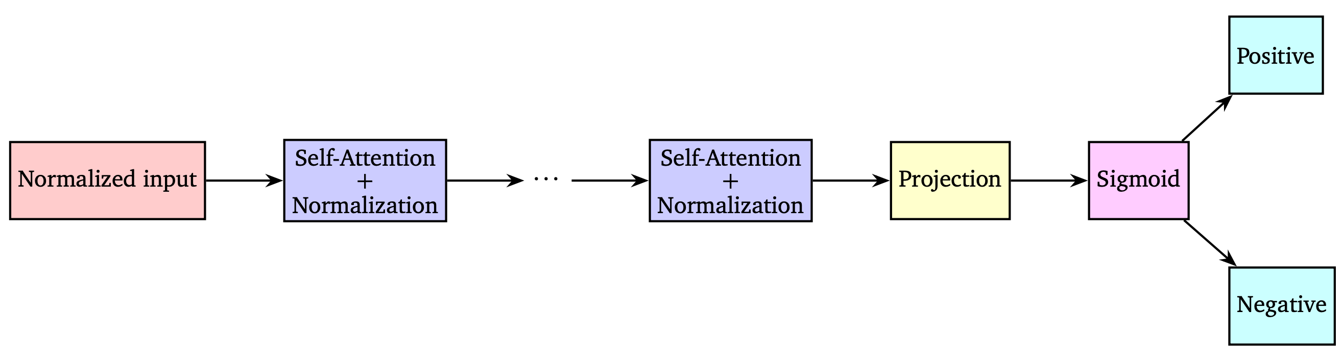
Figure 2. Transformer model without feed forward layers for binary classification

Figure 3 shows the accuracy obtained with several models.

Figure 3. Accuracy for several models

As expected, using $V_k = \alpha_k$ with $\alpha_k \geq 0$ is not very effective.

However, using $V_k = -\alpha_k I_d$ leads to rather good results, especially when we allow the coefficients $\alpha_k$ to depend on $k$ .

Note that when using a basic Neural Network (NN), the results are not bad, but they are below what can be obtained using self-attention. The point of using a NN here is to show that the embedding does not explain all the results, despite the fact that the embedding may learn which words are positive or negative.

Finally, we see that using self-attention and neural networks (or feed-forward layers) leads to the best accuracy here.

Conclusion

The goal of this post was to show that self-attention is a complex mechanism, for which theoretical results can be hard to obtain.

Numerical experiments led us to a few conjectures, which remain to be proved. Moreover, these experiments also showed that performance is increased when using feed-forward layers as well as self-attention layers, which is something else that could be theoretically studied.

References

[1] N. Shazeer, N. Parmar, J. Uszkoreit, L. Jones, A.N. Gomez, L. Kaiser, I. Polosukhin (2017) Attention is all you need. Advances in neural information processing systems 30, https://doi.org/10.48550/arXiv.1706.03762
[2] B. Geshkovski, C. Letrouit, Y. Polyanskiy, P. Rigollet (2023) A mathematical perspective on Transformers, https://doi.org/10.48550/arXiv.2312.10794
[3] J. G. Wendel (1962) A Problem in Geometric Probability. Mathematica Scandinavica, Vol. 11, No. 1, pp. 109-111, https://www.jstor.org/stable/24490189
[4] J. Devlin, J. Devlin, M.W. Chang, K. Lee, K. Toutanova (2018) Bert: Pre-training of deep bidirectional transformers for language understanding, Vol. 1, pp. 4171–4186, arXiv:1810.04805, https://doi.org/10.18653/v1/N19-1423
[5] A.L. Maas, R.E. Daly, P.T. Pham, D. Huang, A.Y. Ng, C. Potts. (2011) Learning Word Vectors for Sentiment Analysis. Proceedings of the 49th Annual Meeting of the Association for Computational Linguistics: Human Language Technologies, pp. 142-150 https://aclanthology.org/P11-1015/