Stability of hyperbolic systems with non-symmetric partial dissipation

Introduction

In this post, we report new results for $n$ -components linear hyperbolic systems in $\R$ of the type

$\partial_tU + A\partial_xU+BU=0. (1)$

The unknown $U=U(t,x)\in \R^{n}$ ( $n\geq2$ ) depends on the time variable $t\in \R_+$ and on the space variable $x\in\R$ , $A$ is a symmetric $n\times n$ matrix and $B$ is a semidefinite positive $n\times n$ matrix such that $rank(B) \lt n$ .

System (1) corresponds to the linearization around constant equilibria of classical hyperbolic systems, such as the compressible Euler equations, the Euler-Maxwell equations, the Timoshenko model, coupled transport equations, the Sugimoto equation, the damped wave equation, and conservation laws.

1.1 Stability in the case $B$ symmetric

The stability of system (1) has been largely studied when the matrix $B$ is symmetric [5,1,2]. In this case, $B$ is dissipative but since rank $(B) \lt n$ , its dissipative effects do not affect every component of the solution. It is always possible to reformulate the system (1) to have

$B = \begin{pmatrix} 0 & 0 \\ 0 & D \end{pmatrix},$

where $D$ is a $n_1\times n_1$ matrix such that rank $(B)=n_1$ with $1\leq n_1 \lt n$ .

In [1], Beauchard and Zuazua show that the Kalman rank condition from control theory is a necessary and sufficient condition to ensure the $L^2$ -stability of (1) i.e. that the $L^2$ -norm of the solutions of (1) decay to zero as time goes to infinity.

Proposition 1.1
For $A$ and $B$ two symmetric matrices, the following statements are equivalent.
• System (1) behaves asymptotically as the heat equation: it is polynomially stable:

$\|U(t)\|_{L^2}\leq (1+t)^{- \frac12}\|U_0\|_{L^2\cap L^1} (2)$

• The pair $(A,B)$ satisfies the Kalman rank condition:
(Kalman rank condition:) the matrix:

$\mathcal{K}(A,B):=(B,BA,\ldots,BA^{n-1})^T\quad$

has full rank $n$ .

Such a result exploits the Kalman rank condition to ensure that every component is dissipated, using interactions between the hyperbolic part $A$ and the dissipative part $B$ .
Idea of the proof.
Applying the Fourier transform to (1), we obtain the parameterized ODE

$∂_t\widehat{U}+i\xi A \widehat{U}+B\widehat{U}=0, (3)$

where $\xi\in\R$ is the frequency parameter.
A key observation is that for $\xi=1$ the system becomes an ODE for which the exponential stability of the solutions of (3) is equivalent to the Kalman rank condition for the pair $(A,B)$ .
Such a result, established for instance in [3], shows that stability results for ODEs can be proved even if the rank of the dissipative matrix is not full.
Similar results can be obtained for our hyperbolic system (1), except that the stability is not exponential due to the parameter $\xi$ . In [1], Beauchard and Zuazua used the augmented Lyapunov functional

$\mathcal{L}(t)=|\widehat{U}|^2+\min(1/|\xi|,|\xi|) {\rm Re} \sum_{k=1}^{n-1} \varepsilon_k \langle BA^{k-1}\widehat{U}\cdot BA^k\widehat{U} \rangle, (4)$

where the $\varepsilon_k$ parameters are chosen small enough to ensure coercivity. The main difference with the ODE framework is that the value of the parameter $\xi$ influences drastically the behaviour of the system. Roughly, one sees that for $|\xi|\ll 1$ the dissipative part is dominant in (3)
and for $|\xi|\gg 1$ the hyperbolic part dominates. To resolve this complication, in [1], the authors include the frequency weight $\min(1/|\xi|,|\xi|)$ in the augmented energy functional (4) (compared to the ODE framework) so that the dissipative and hyperbolic operators are at the same frequency scale and can interact. Then, differentiating in time (4) and using that the Kalman rank condition implies that

$\bigg(\sum_{k=0}^{n-1} |BA^{k}y|^2\bigg)^{\frac{1}{2}} (5)$

defines a norm for any $y\in \mathbb{C}$ , one obtains

$|\widehat{U}(\xi,t)|^2\leq C|\widehat{U_{0}}(\xi)|^2e^{-c\min\{1,|\xi|^2\}t}. (6)$

The inequality (6) leads to desired stability result and the dichotomous behaviour:
• The high frequencies of the solutions are exponentially damped,
• The low frequencies behave like the heat equation.
In other words, solutions to equation (1) satisfy

$\|\widehat U^h(t)\|_{L^2} \leq Ce^{-\gamma t}\|\widehat U^h_0\|_{L^2}, (7) \\ \|\widehat U^\ell(t)\|_{L^2} \leq Ct^{-\frac{1}{4}}\|\widehat U^\ell_0\|_{L^2}, (8)$

where $C$ and $\lambda$ are positive constants depending on $A$ and $B$ , $U^h(\xi,t)=\widehat U(\xi,t)\mathbf{1}_{|\xi|\geq1}$ and $U^\ell(\xi,t)=\widehat U(\xi,t)\mathbf{1}_{|\xi|\leq1}$ .

Case $B$ non-symmetric

Up to this point, we have assumed the matrix $B$ is symmetric, which is a well-understood case. We now turn our attention to the case where $B$ is not symmetric, which is much less studied. It turns out that taking a closer look at this case can yield surprising results which can be applied to physical models such as the Timoshenko beam model or the compressible Euler-Maxwell system.

1.2 Stability of ODEs

Before discussing the PDE setting, let us quickly look at ODEs. We consider

$\dot{X}+AX=-BX, (9)$

where $A$ is a skew-symmetric matrix, $B$ is non-symmetric and $B\geq0$ i.e. positive semidefinite. To study the stability of (9), since the skew-symmetry of $A$ implies that it corresponds to the conservative part, the first step is to identify the subspace where $B$ is dissipative. In practice, this is given by its symmetric part $B^s$ defined as $B^s=\frac{1}{2}(B+B^T)$ . The subspace where $B$ is dissipative can be slightly more general than this but we will restrict ourselves to the symmetric part here.
Then, rewriting the system as

$\dot{X}+(A+B^a)X=-B^sX,$

where $B^a=\frac12(B-B^T)$ and $B=B^s+B^a$ , the stability of (9) is equivalent to $(A+B^a,B^s)$ satisfying the Kalman rank condition.
If one does not separate the dissipative and conservative parts clearly then it does not make sense to involve the Kalman rank condition.
For instance, for

$B=\begin{pmatrix} 0 & 1 & 0 \\ -1 & 0 & 0 \\ 0 & 0 & 1 \end{pmatrix},$

we have rank( $B$ )=3 and the Kalman rank condition would always hold, but this does not yield any time-decay results as $B$ only brings dissipation on the component $U_3$ .
However, considering

$A=\begin{pmatrix} 0 & 0 & 0 \\ 0 & 0 & 1 \\ 0 & 1 & 0 \end{pmatrix}, \quad B=\begin{pmatrix} 0 & 1 & 0 \\ -1 & 0 & 0 \\ 0 & 0 & 1, \end{pmatrix}$

we can use that $(A+B^a,B^s)$ verifies the Kalman rank condition to derive the exponential stability as $B^s$ is purely dissipative. Notice that in this example the couple $(A,B^s)$ does not satisfy the Kalman rank condition and therefore the skew-symmetric part of $B$ is essential to justify the exponential stability. This fact will be of great importance in the context of PDEs, when the operators are of a different order.

2.2 Heuristics in the PDE setting

A similar approach can be used to analyse the stability of partially dissipative hyperbolic systems. Consider

$\partial_t U + A\partial_xU =-BU (10)$

where $A$ is a skew-symmetric matrix, $B$ is non-symmetric and $B\geq 0$ . Applying the Fourier transform and decomposing $B=B^s+B^a$ , we rewrite the system as

$∂_t \widehat{U}+(i\xi A+B^a)\widehat{U}=-B^s\widehat{U}. (11)$

In the context of PDEs, the main difficulty compared to the ODE setting is that the operators $A\partial_x$ and $B$ cannot directly interact with each other, as their orders differ. To overcome this problem one has to include frequency weights in the computations, just like in (4), so that the operators can communicate. Here, however, the situation is a bit different and rewriting (10) as (11) allows for more complex interactions depending on the frequency-regime under consideration. For instance, for low frequencies ( $|\xi|\ll 1$ ) one observes that the term $B^a$ becomes the dominant skew-symmetric part, so if $(B^a,B^s)$ satisfies the Kalman rank condition then one simply expects exponential stability as in the ODE setting.
One can identify multiple scenarios that may occur when studying the stability of (10).

(i) Classical PDE condition: $(A,B)$ satisfies the Kalman rank condition and $B$ is symmetric $\rightarrow$ the solutions satisfy (7)-(8).

(ii) ODE-type condition: $(B^a,B^s)$ satisfies the Kalman rank condition $\rightarrow$ the system is exponentially stable.

(iii) Classical PDE condition v2: $(A,B^s)$ satisfies the Kalman rank condition $\rightarrow$ the solutions satisfy (7)-(8).

(iv) Low frequencies improvement: Both $(A,B^s)$ and $(B^a,B^s)$ satisfy the Kalman rank condition $\rightarrow$ the system is exponentially stable.

(v) The skew-symmetric part complements the lack of dissipation: Neither $(A,B^s)$ or $(B^a,B^s)$ satisfy the Kalman rank condition but interaction between $B^a$ and $B^sA^k$ , for $0\leq k \leq n-1$ , are needed $\rightarrow$ the solutions is stable in a weaker sense, cf Section 2.3.

These scenarios can occur in multiple physical applications. The next section briefly presents the last one.

2.3 A concrete example for scenario (v): The Timoshenko-Cattaneo system

We now focus on a system for which exploiting the skew-symmetric part of $B$ is crucial to establish stability results. We look at the Timoshenko-Cattaneo system reformulated in a first-order hyperbolic system as in [4, p.24]. It reads

$\left\lbrace \begin{array}{ll} ∂_{t}u_1-∂_xu_3+u_2=0, \\ ∂_tu_2-a∂_xu_4+b∂_xu_5-u_1=0, \\ ∂_tu_3-∂_xu_1=0, \\ ∂_tu_4-a∂_xu_2=0, \\ ∂_tu_5+b∂_xu_2+\sqrt{\kappa}∂_x u_6=0 \\ \varepsilon∂_t u_6+\sqrt{\kappa}∂_x u_5+u_6=0 \end{array} \right. (12)$

For (12), the associated matrix read

$A=\begin{pmatrix} 0 & 0 & -1 & 0 & 0 & 0 \\ 0 & 0 & 0 & -a & b & 0 \\ -1 & 0 & 0 & 0 & 0 & 0 \\ 0 & -a & 0 & 0 & 0 & 0 \\ 0 & b & 0 & 0 & 0 & \sqrt{\kappa} \\ 0 & 0 & 0 & 0 & \sqrt{\kappa} & 0 \\ \end{pmatrix} B=\begin{pmatrix} 0 & 1 & 0 & 0 & 0 & 0 \\ -1 & 0 & 0 & 0 & 0 & 0 \\ 0 & 0 & 0 & 0 & 0 & 0 \\ 0 & 0 & 0 & 0 & 0 & 0 \\ 0 & 0 & 0 & 0 & 0 & 0 \\ 0 & 0 & 0 & 0 & 0 & 1 \\ \end{pmatrix} (13)$

where the matrix $A$ is symmetric but the matrix $B$ is not. Let us now apply the reasoning from the previous sections.

• First, we need to identify in which subspaces is the matrix $B$ strongly dissipative. Clearly, it is the symmetric part $B^s$ that is dissipative and it only affects the component $u_6$ .

• Now, we check if standard Kalman-type conditions are satisfied. To justify the stability of (12), we see that it is not enough to use Kalman-type interactions between $B^s$ and $A$ or $B^s$ and $B^a$ as the pairs $(A,B^s)$ and $(B^a,B^s)$ do not satisfy the Kalman rank condition. Indeed, their interactions would only lead to dissipation for the components $u_2,u_4,u_5$ and $u_6$ .

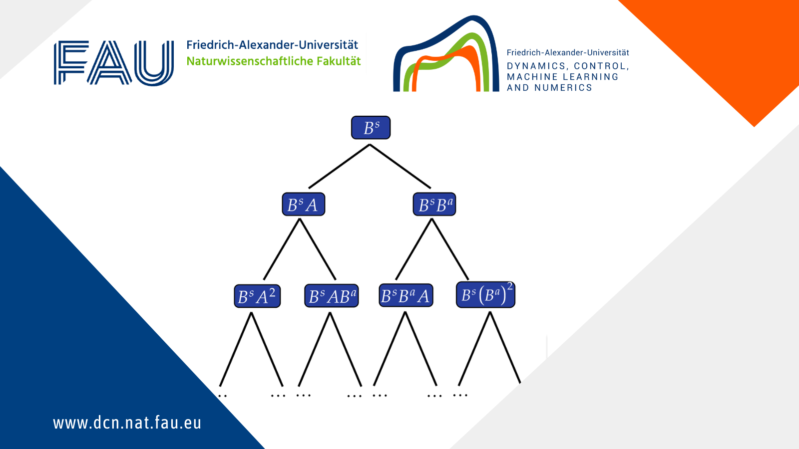
To stabilize the components $u_1$ and $u_2$ , one must use interactions between $B^sA^k$ and $B^a$ . Roughly, the Kalman-type procedure goes as follows:
(1) Im $(B^s) \rightarrow$ dissipation for $u_6$ .

(2) Im $(B^sA) \rightarrow$ dissipation for $u_5$ .

(3) Im $(B^sA^2) \rightarrow$ dissipation for $u_2$ .

(4) Im $(B^sA^3) \rightarrow$ dissipation for $u_4$ .

(5) Im $(B^sA^2B^a) \rightarrow$ dissipation for $u_1$ .

(6) Im $(B^sA^2B^aA) \rightarrow$ dissipation for $u_3$ .

However, due to the difference in the order of $A\partial_x$ and $B^a$ , the procedure is more complex and one needs to decompose the frequency space into the low and high-frequency. In the end, we are not able to justify the exponential decay of the solutions nor the classical polynomial stability as in case $B$ symmetric (7)-(8).
Denoting $U=(u_1,u_2,u_3,u_4,u_5,u_6)$ , under certain conditions on $a,b$ and $\kappa$ , specified in [4], it is possible to show that

$|\widehat{U}(t)|^2\lesssim e^{\lambda_{\varepsilon}(|\xi|)t}|\widehat{U}_0|^2,\quad\quad t>0,\quad \xi\in\R, (14)$

where $\lambda_{\varepsilon}(|\xi|)$ is given by

$\lambda(|\xi|)=-\frac{|\xi|^4}{(1+|\xi|^2)^3}, (15)$

Such an inequality implies stability, but for high frequencies we have $\lambda(|\xi|)\sim 1/|\xi|^2$ for $|\xi|\gg1$ which implies a loss of derivatives: for $H^k$ data, with $k\geq 2$ , we recover time-decay estimates in $H^{k-2}$ .
In low frequencies ( $|\xi|\ll 1)$ , we have $\lambda(|\xi|)\sim |\xi|^4$ and we recover a bi-laplacian behavior in this regime.

If we assume that for $k,\ell>0$ we have $U_0\in H^{k+\ell}\cap L^1;$ then, for all $t>0$ , we get the following decay estimates for (12)

$\| ∂_x^kU^h(t)\|_{L^2} \leq (1+t)^{-\frac{\ell}{2}}\| ∂_x^{k+\ell} U^h_0\|_{L^2}, (16) \\ \|∂_x^kU^\ell(t)\|_{L^2} \leq Ct^{-\frac{1}{8}-\frac{k}{4}}\| U^\ell_0\|_{L^1}, (17)$

Overall (16) and (17) lead to weaker decay rates in both regimes compared to the case $B$ symmetric, but without using the interactions between $B^s$ , $A$ and $B^a$ it would not have been possible to justify the stability at all. The key point to remember is that Kalman-type conditions are also useful in the PDE setting to justify stability results but the decay estimates that one recovers will depend on the difference between the order of each operator involved in Kalman-type interactions and the way these interactions occur.

Remark 2.1 An extension: Heuristics in the case $A$ non-symmetric.
A natural follow-up question is what happens when the matrix $A$ is not symmetric. Using the decomposition $A=A^s+A^a$ , we get
$∂_t \widehat{U}+(i\xi A^s+B^a)\widehat{U}=(i\xi A^a+B^s)\widehat{U}.$ If $A^a$ is positive definite, then we expect that the skew-symmetric part of $A$ could provide additional time-decay information. For instance, if $(A^s,A^a)$ satisfies the Kalman rank condition, then one expects to recover improved time-decay rates in high frequencies. This example is mainly academic as an explicit example of a PDE modelling physical phenomenon seems out of reach.

References

[1] K. Beauchard and E. Zuazua. Large time asymptotics for partially dissipative hyperbolic systems. Arch. Ration. Mech. Anal, 199:177–227, 2011.
[2] T. Crin-Barat and R. Danchin. Partially dissipative hyperbolic systems in the critical regularity setting : The multi- dimensional case. J. Math. Pures Appl. (9), 165:1–41, 2022.
[3] R. E. Kalman, P. L. Falb, and T. M. A. Arbib. Topics in Mathematical Control Theory, volume New York-Toronto, Ont.-London. 1969.
[4] N. Mori. An S&K mixed condition for symmetric hyperbolic systems with non-symmetric relaxations. Article in European Journal of Mathematics, 2019.
[5] S. Shizuta and S. Kawashima. Systems of equations of hyperbolic-parabolic type with applications to the discrete Boltzmann equation. Hokkaido Math. J., 14, 249-275, 1985.