
Controllability properties of fractional PDE
Umberto Biccari, DeustoCCM
Controllability of the fractional heat equation
Let \omega\subset (-1,1) be an open and nonempty subset. Consider the following non-local one-dimensional heat equation defined on the domain (-1,1)\times(0,T)
\begin{cases} y_t + (-d_x^2){^s}{y} = u\mathbf{1}_{\omega},\quad & (x,t)\in (-1,1)\times(0,T) \\ y=0, & (x,t)\in(-1,1)^c\times(0,T) \\ y(x,0)=y_0(x), & x\in (-1,1), \end{cases}
where y_0\in L^2(-1,1) is a given initial datum. In (1), for all s\in(0,1), \fl{s}{} denotes the one-dimensional fractional Laplace operator, which is defined as the following singular integral
(-d_x^2){^s}{y}(x) = c_s\,P.V.\,\int_{\R}\frac{y(x)-y(\xi)}{|x-\xi|^{1+2s}}\,d\xi.
Here, c_s is the following explicit normalization constant
c_s = \frac{s2^{2s}\Gamma\left(\frac{1+2s}{2}\right)}{\sqrt{\pi}\Gamma(1-s)},
where \Gamma is the usual Gamma function.
It has been shown in [4] that the fractional heat equation (1) enjoys the following controllability properties.
Theorem 1. Given any y_0\in L^2(-1,1), the parabolic problem (1) is null-controllable at time T>0 with a control function u\in L^2(\omega\times(0,T)) if and only if s>1/2.
Theorem 2. Given any y_0\in L^2(-1,1), the parabolic problem (1) is approximately controllable at time T>0 with a control function u\in L^2(\omega\times(0,T)) for any s\in(0,1).
The proof of Theorem 1 is carried out with spectral techniques. It is a consequence of the following asymptotic behavior of the eigenvalues od the Dirichlet fractional Laplacian (see [8])
\lambda_k = \left(\frac{k\pi}{2}-\frac{(1-s)\pi}{4}\right)^{2s}+O\left(\frac{1}{k}\right).
and of the Müntz condition ensuring that null-controllability holds if and only if
\sum_{k\geq 1} \frac{1}{\lambda_k}<+\infty.
Theorem 2, instead, follows from the unique continuation property of the fractional Laplacian obtained in [6].
Computation of the optimal control – the penalized Hilbert Uniqueness Method
By means of the so-called penalized Hilbert Uniqueness Method (HUM) and of the Fenchel-Rockafellar duality theory (see [5]), the control of minimal L^2(\omega\times(0,T)) norm for the fractional heat equation (1) can be computed as follows:
Step 1. we solve the minimization problem
\widehat{p}^{\,T}_{\varepsilon} = \min_{p_T\in L^2(-1,1)} J(p^T) \\ J(p^T) = \frac{1}{2}\int_0^T{||p(\cdot,t)||}{L^2(-1,1)}^2\,dt+\frac{\varepsilon}{2}{||p^T||}{L^2(-1,1)}^2 + \langle z(\cdot,T),p^T\rangle
where p is the solution of the adjoint equation
\begin{cases} -p_t + (-d_x^2){^s}{p} = 0,\quad & (x,t)\in (-1,1)\times(0,T) \\ p=0, & (x,t)\in(-1,1)^c\times(0,T) \\ p(x,T)= p^T(x), & x\in (-1,1). \end{cases}
and z is the solution of the uncontrolled equation
\begin{cases} z_t + (-d_x^2){^s}{z} = 0,\quad & (x,t)\in (-1,1)\times(0,T) \\ z=0, & (x,t)\in(-1,1)^c\times(0,T) \\ z(x,T)=y_0(x), & x\in (-1,1). \end{cases}
Step 2. Then, the control for (1) is given by
u_\varepsilon = \widehat{p}_\varepsilon\;\mathbf{1}_\omega,
with \widehat{p}_\varepsilon solution of (4) corresponding to the initial datum \widehat{p}^{\,T}_\varepsilon.
Moreover, the approximate and null controllability properties of (1) can be characterized in terms of the behavior of the penalized HUM approach with respect to the parameter \varepsilon. In particular, we have (see [5], Theorem 1.7])
1. Problem (1) is approximately controllable from the initial datum z_0 if and only if
y_\varepsilon(\cdot,T)\to 0,\;\;\;\textrm{ as }\;\varepsilon\to 0,
where y_\varepsilon is the solution corresponding to the optimal control latex]u_\varepsilon[/latex].
2. Problem (1) is null-controllable from the initial datum y_0 if and only if
M_{y_0}^2:=2\sup_{\varepsilon>0}\left(\sup_{L^2(-1,1)}J\right)<+\infty.In this case, we have
||{u_\varepsilon}||{L^2(\omega\times(0,T))}\leq M_{y_0}, \\ ||{y_\varepsilon(\cdot,T)||}{L^2(-1,1)}\leq M_{y_0}\sqrt{\varepsilon}.
To corroborate the theoretical results Theorems 1 and 2, we solved numerically the optimization problem (3). The minimization of the functional is carried out with a standard Conjugate Gradient algorithm (see for instance [7]). The underneath dynamics is simulated employing FE for the approximation of the fractional Laplace operator on a uniform mesh of size h (see [4] for more detail on how to compute the stiffness matrix) and an implicit Euler scheme on a M-points uniform partition of (0, T).
The control region is \omega=(-0.3,0.8) and the time horizon for control is T=0.3s. As initial datum we chose y_0 = \sin(\pi x).
Figure 1 shows the behavior of the penalized HUM with respect to \varepsilon, in the case s = 0.8 in which null controllability is expected. Here, following [5] we selected \varepsilon = h^2. We can observe that the cost of the control and the optimal energy M_{y_0} remain bounded as h → 0. Moreover, the target y_\varepsilon(\cdot,T) tends to zero with a rate \sqrt{\varepsilon}=h. This confirms that (1) is indeed null-controllable.
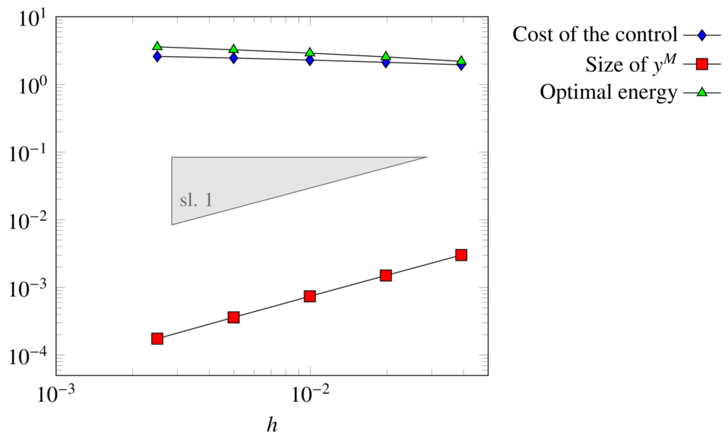 Figure 1. Behavior with respect to \varepsilon = h^2 of the penalized HUM in the case s = 0.8
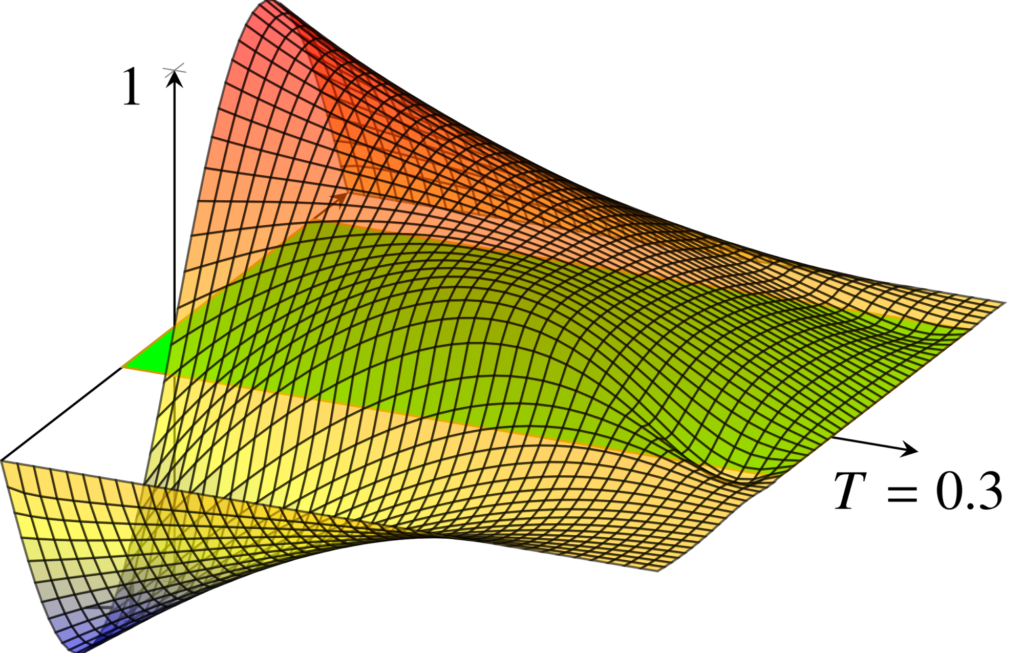
Figure 2 shows the time evolution of the solution of (1) without and with the action of the optimal control computed through the previous methodology. We can see how the introduction of a control allows us to steer the solution to zero at time T.


Figure 2. Evolution of the free (left) and controlled (right) dynamics of (1)
Finally, Figure 3 shows the behavior of the penalized HUM with respect to \varepsilon, in the cases s=0.4 and s=0.5. We can observe that the results here are different than the ones of Figure 1. In particular, both the cost of the control and the optimal energy M_{y_0} increase as as h\to 0. Moreover, the target y_\varepsilon(\cdot,T) tends to zero with a rate slower than \sqrt{\varepsilon}. This confirms that (1) is only approximately-controllable.
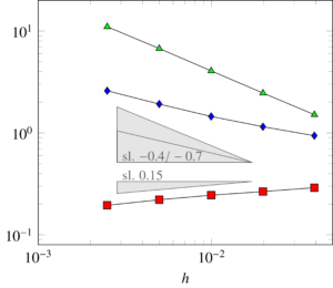
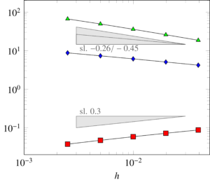
Figure 3. Behavior with respect to \varepsilon = h^2 of the penalized HUM in the cases s=0.4 (left) and s=0.5 (right)
More complete details on the topics of this post can be found in [4]. We also refer to [1, 2, 3] for other theoretical and numerical results on controllability properties of PDE involving the fractional Laplacian.
References
[1] H. Antil, U. Biccari, R. Ponce, M. Warma and S. Zamorano, Controllability properties from the exterior under positivity constraints for a 1-D fractional heat equation, submitted
|| Go to the Math & Research main page


