
Classical models
Cyprien Neverov, FAU DCN-AvH
Download Data-Driven COVID Modeling (Slides)
Compartmental epidemiological models [1] were introduced almost a century ago and are still considered the standard way of modeling a disease in a population.
They are also called SIR models because they divide the population into different compartments like Susceptible, Exposed, Infected, Recovered and model the interactions between the compartments.
For example the simplest SIR model is governed by the following ODE:

where N is the total population and \gamma, \beta are the parameters of the disease.
Other approaches for modeling the spread of an infectious disease include:
- Spatiotemporal SIRs are the most obvious extension of the SIR models to include interactions in space. This is achieved by dividing the total population into areas and adding a spatial term to model regional processes [3, 4].
- Statistical models are more inclined towards capturing the random nature of the infectious diseases. Thorough reviews of these approaches can be found in [5] and [6].
- Gravity models can be used as standalone models or in conjunction with the compartmental approach and are called “gravity” models because they rely on considering the effect of distance and the size of donor and recipient communities [7, 8].
- Network-based models are built on the assumption that the spread of human disease follows its specified contact or spreading paths such as transportation or social contact networks [9, 10]
- Agent-based models are based on the belief that individuals and their mutual differences are the key to understanding the spread of an infection [11, 12].
Additionally, hybrid approaches combining different methods are considered in the literature [13, 14] as well as more computationally-oriented methods like cellular automata [15]. A thorough review about the modeling of infectious diseases can be found in [16].
Data driven approach
We decided to take an approach without this domain knowledge and explore the usage of a system identification tool called Sparse Identification of Nonlinear Dynamics [2] that allows to find an ODE from observed data.
This system identification algorithm has two key features: (1) it relies on a set of user-defined candidate functions and (2) it converges to a sparse formulation of the dynamics by gradually zeroing-out the values that are under a certain threshold.
The simplest way of using system identification for COVID is by finding the dynamics that govern the evolution of the cumulative cases in a given country. If we call \mathbf{x}_t the cumulative number of cases at day t then, what we want to find is a function f such that:
\mathbf{x}_{t+1} = f(\mathbf{x}_t)
As candidate functions we can for example use polynomial terms of the state. This allows us to reformulate the problem and say that we are looking for optimal \alpha_0, \alpha_1, \alpha_2, ..., \alpha_n such that:
\mathbf{x}_{t+1} = \sum_{k=0}^n \alpha_k \mathbf{x}_t^k
where n is the maximum degree of the polynomial terms.
Sparse Identification of Nonlinear Dynamics
Now let’s take a closer look at the algorithm that is the core of this approach.
As mentioned earlier, it relies on candidate functions and searches for a sparse formulation of the dynamics. Here we are going to describe the three main steps of this algorithm, applied to the aforementioned problem.
From this example it will be quite easy to generalize to other cases.
1. Since the data for a dynamic system is a series of observations at different times (\mathbf{x}_1, \mathbf{x}_2, \mathbf{x}_3, ..., \mathbf{x}_T), we need to divide the data into two matrices X_2 and X_1 which will then allow us to easily formulate an optimization problem:
X_2 = \begin{bmatrix} \mathbf{x}_2 \\ \mathbf{x}_3 \\ \vdots \\ \mathbf{x}_T \end{bmatrix} \text{ and } X_1 = \begin{bmatrix} \mathbf{x}_1 \\ \mathbf{x}_2 \\ \vdots \\ \mathbf{x}_{T-1} \end{bmatrix}
2. The second step consists in augmenting the X_1 matrix with the candidate functions, we will call this matrix \theta(X_1) as in the original paper. Here we use polynomial terms as candidate functions but in a more general case all kind of functions can be used.
\theta(X_1) = \begin{bmatrix} X_1^0 & X_1^1 & X_1^2 & \cdots & X_1^n \end{bmatrix} = \begin{bmatrix} 1 & \mathbf{x}_1 & \mathbf{x}_1^2 & \cdots & \mathbf{x}_1^n\\ 1 & \mathbf{x}_2 & \mathbf{x}_2^2 & \cdots & \mathbf{x}_2^n\\ \vdots & \vdots & \vdots & \ddots & \vdots\\ 1 & \mathbf{x}_{T-1} & \mathbf{x}_{T-1}^2 & \cdots & \mathbf{x}_{T-1}^n\\ \end{bmatrix}
3. The last step is the actual optimization: now we are looking for a matrix \xi = \begin{bmatrix} \alpha_0 \\ \alpha_1 \\ \vdots \\ \alpha_n \end{bmatrix}that solves the following equation in the least squares sense:
And then we can reiterate this optimization a few times and at each iteration remove the candidate functions whose coefficient has an absolute value under a certain threshold called cutoff value.
For example assuming a maximum degree of 4 and using this method on COVID data of cumulative cases in Germany available on May 7th, 2020 would give the following results:
\mathbf{x}_{t+1} = 4.07 \times 10^{-3} + 1.24 \times \mathbf{x}_t - 3.33 \times 10^{-2} \times \mathbf{x}_t^2 + 1.66 \times 10^{-3} \times \mathbf{x}_t^3 - 3.21 \times 10^{-5} \times \mathbf{x}_t^4
The following figure shows the integration of this model and its comparison to the real data.
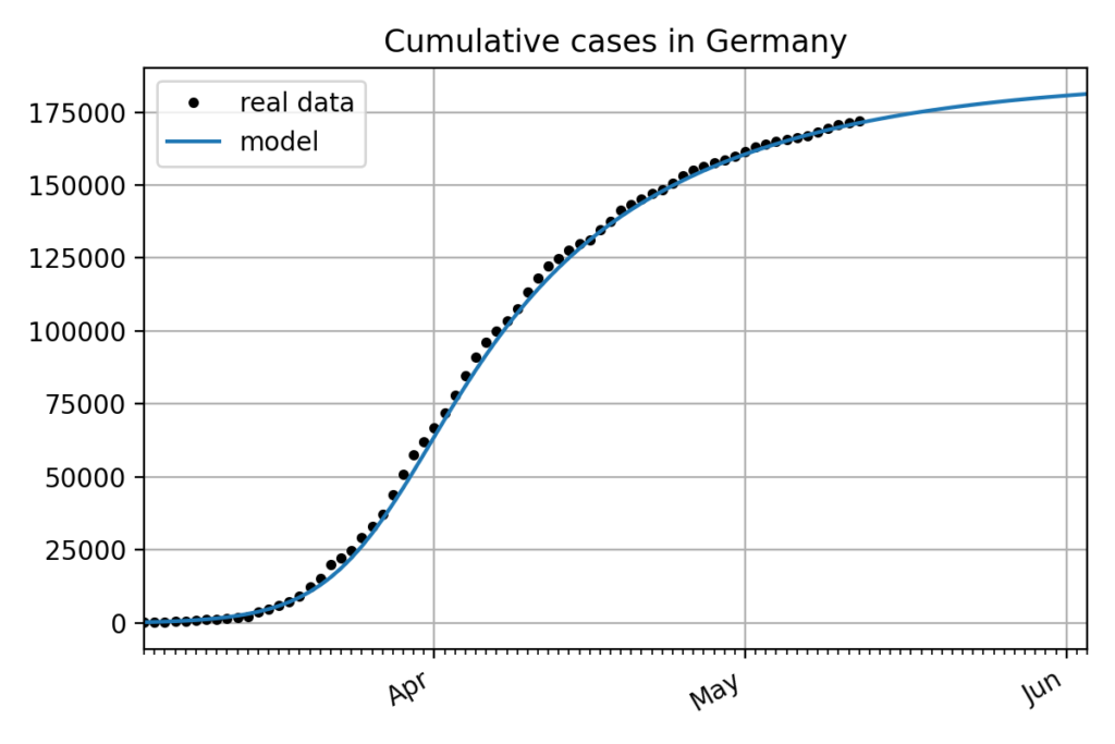
Even if the model perfectly fits the data in this particular example about the cumulative cases in Germany, trying on different countries shows that the influence of the different parameters as well as other variables like the noise in the data is not well understood.
Cutoff value
For this particular case the cutoff value was extremely small to allow the model to have its maximum complexity because is has only 5 candidate functions and the resulting formula doesn’t need to be sparse because it is still completely understandable to humans.
But the cutoff value is a very important parameter when the number of candidate functions is bigger.
For example if we consider a Lorenz attractor, it will have three variables, one for every dimension of the space and if we use polynomials of a maximum degree of 4 and use all possible polynomial terms then we end up with 21 candidate functions and obviously we don’t want all the coefficients to be non zero.
Instead, what is desired is the simplest formulation that fits the data and a carefully chosen cutoff value can allow us to reach this goal.
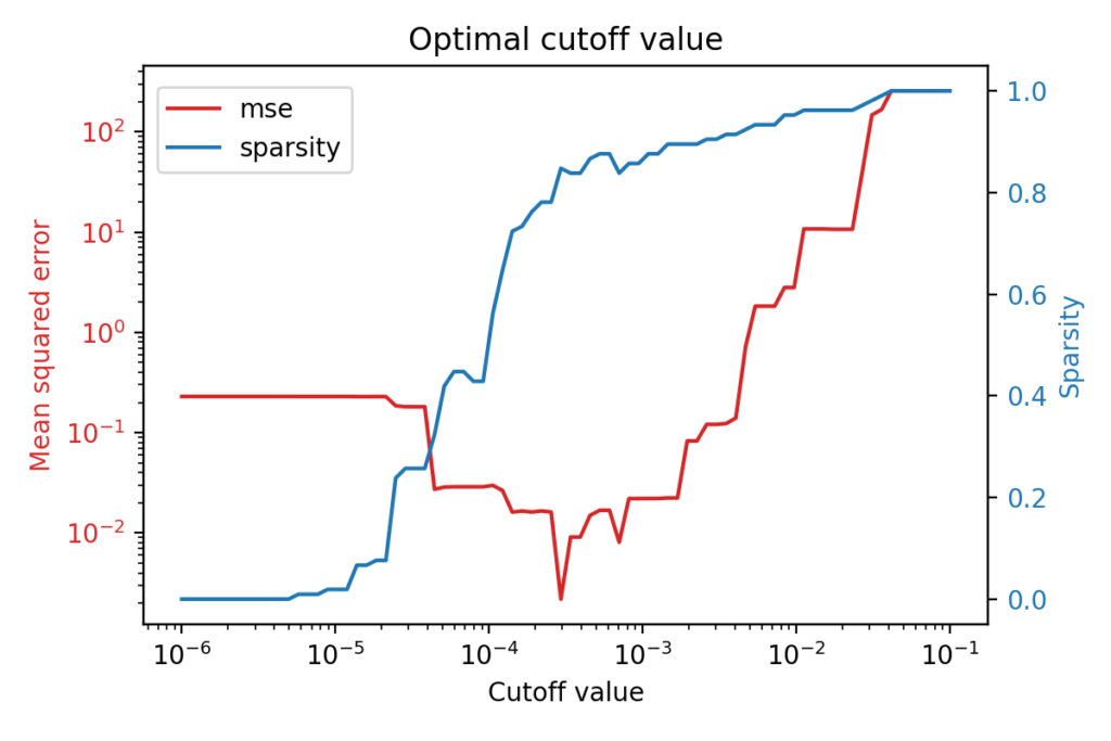
The figure above shows that there is an optimal cutoff value for the identification of a Lorenz system from observed data. The red line shows the mean squared error of the model with respect to the cutoff value, while the blue one shows how sparse the model is for this particular cutoff value.
What is interesting is that the best performing model is not the most complex one but rather a very sparse one: less than 20% of the coefficients are non-zero, thus the optimal cutoff value for this case is around 3 \times 10^{-4}
Similarly, when exploring the dynamics that can be identified from the COVID-19 data and any additional information that we might want to add, it is important to understand the effects of parameters like the cutoff value or the maximum degree of the polynomial terms.
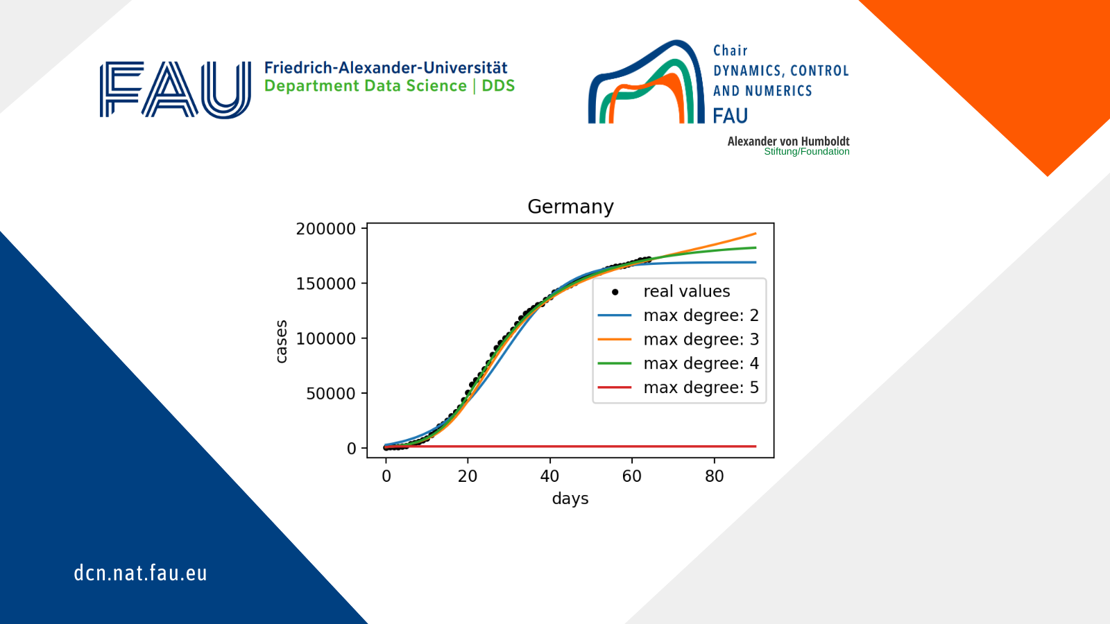
As depicted in the figure below, the maximum degree can also have a massive influence on resulting models.
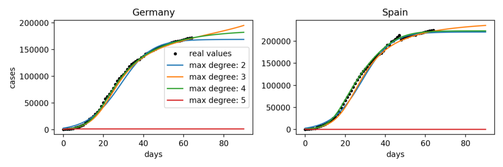
Indeed, we can observe that for Germany the most realistic model uses polynomials of a maximum degree of 4 while for Spain it is the one with polynomial terms with a maximum degree of 3. Doing this fitting on a bigger number of countries suggests that there is no maximum degree that gives consistently better results than others. We can also notice that for some reason, with a maximum degree of 5 the model no longer works for both these countries.
Predictive power
One other aspect that is very interesting to develop in the scope of this system identification approach is forecasting. When considering the simple modeling of the number of cumulative cases in a single country like we did for Germany, we observed that with the right set of parameters we were able to identify dynamics that are very close to reality. But obviously this fitting doesn’t imply that the model will do good extrapolation.
In order to evaluate the forecasting accuracy of identified dynamics we compared identified models with different parameters to a classic statistical forecasting model, namely autoregressive integrated moving average (ARIMA).
In fact, from the so-far available literature on COVID it seems that this model is a common choice for statisticians to do forecasting [17, 18, 19].
An ARIMA(1, 1, 4) was selected and system identification was used with maximum degrees ranging from 2 to 7 and with a very low cutoff value because we are not looking for sparsity in this particular case. The two main reasons are that fitting quality is more interesting to us than sparse formulation and that testing different cutoff values did not show improvements in the results. Using a wide range of maximum degrees allows us to overcome the problem discussed earlier where we do not know for a given country what maximum degree is going to perform best.
The comparison was done on two forecast horizons: one and two weeks. It means that the different models were trained with all the evolution of the cumulative cases except the last two weeks that were used for evaluation. The results were compared using mean squared error. The following figure shows the percentage of countries on which each model did the best predictions.
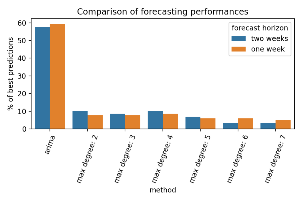
On more than 55% of the 118 considered countries, the ARIMA model showed better forecasting capabilities than the identified dynamical systems. Considering the fact that ARIMA parametrization requires careful handling, it is probably not optimal in our case, yet the statistical model still outperforms the identified models.
This result is not very surprising since we are comparing a forecasting tool to our models that were not specifically designed to have good extrapolation properties, but instead were designed to closely fit training data. One other observation that can done on the figure above is that, as mentioned earlier, there is no maximum degree that performs consistently better than others.
Investigation directions
In addition to the discussion above about forecasting power, the work around this topic will be directed towards better understanding the identification of the dynamics as well as making the model increasingly sophisticated by adding additional information as variables. In order to do so, the following directions can be explored:
- Adding data about country characteristics as well as government control measures to assess the ability of the system identification to find a system that could be valid for several countries and that could generalize to other countries.
- Investigating what kind of dynamics can be identified from observed susceptible, infected and recovered quantities in different countries and how they compare to compartmental models.
Download Data-Driven COVID Modeling (Slides)
References
[1] Kermack, William Ogilvy, A. G. McKendrick, and Gilbert Thomas Walker. 1997. A Contribution to the Mathematical Theory of Epidemics. Proc. R. Soc. Lond. 12: 700–721
|| Go to the Math & Research main page


