
Breaking the curse of dimensionality with Barron spaces

1 Introduction
Recent advances in computational hardware have enabled the implementation of the set of algorithmic methods known as Deep Learning, whose development nevertheless dates back several decades. In this way, they have emerged in the latest years as the main tool in many practical Machine Learning problems, especially those belonging to the category of Supervised Learning that uses labelled datasets to train algorithms that classify data or predict outcomes accurately. Some of these applications are image analysis, natural language processing or sales forecasting.
However, the unparalleled superior performance of Deep Learning hasn’t found a precise explanation yet. From a theoretical point of view, we still have not passed the initial stages of exploration. Broadly speaking, Deep Learning consists of learning complex representations by repeatedly passing inputs through the layers of a neural network to disentangle their higher-level features. One of the first steps in understanding the source of its power is to characterize the set of problems that a neural network model can learn efficiently.
1.1 Problem statement
In the classical Supervised Learning problem, the main objective is to teach the computer a particular piece of knowledge from a series of examples, as a human being might would learn it. More precisely, the aim is to acquire the ability to identify the class to which each element of a set belongs from a finite number of possibilities (classification problem), or to assign each element to a value from a continuous range (regression problem).
From a mathematical point of view, the problem seeks to approximate an unknown objective function F^* that can label any element (input vector) x of an input space X\subset\mathbb{R}^d to its corresponding label y from the output space Y\subset\mathbb{R}^m. Because of this ideal characterization as an absolute knowledge, it is sometimes called the oracle function.
Remark 1.1
The dimension d is typically very large, while m might take lower values. In fact, we will often consider m=1 throughout this text.
For this purpose, we can only use the information contained in a finite dataset \mathcal{D}=\{(x_i,y_i)\}_{i=1}^N\subset X\times Y, which verifies that y_i=F^*(x_i) for all i=1,\dots,N, and the goal is to obtain a good representation of F^* that can accurately predict the unknown label of any new input. But, how can we construct such a predictive model?
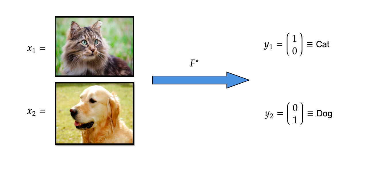 FIGURE 1. Example of an objective function F^* that recognizes whether a given picture from the input space is containing a dog or a cat. Observe that in this classification problem we have m=2 while d takes an extremely large value: the input has one component for each of the pixels of the photograph, and there are three extra dimensions for each pixel to represent its color.
1.2 Learning procedure
The process to construct the predictive model \hat F is called the learning procedure. However, it is not clear where we can even look for it. Consequently, this motivates the first step of the method: limiting the search to a fixed parameterized class of functions called the hypothesis space \mathcal{H}_\theta and choosing inside it the function \hat F\in\mathcal{H}_\theta that “best approximates” F^* as our learned model.
How can we take \hat F among all the functions in the hypothesis space? This is the second step of the learning procedure, and consists in the minimization of a functional that measures the closeness between F^* and the possible models F_\theta\in\mathcal{H}_\theta.
Ideally, the best possible predictor in \mathcal{H} would be obtained through population risk minimization:
\text{argmin}_{F_\theta\in\mathcal{H}_\theta}\mathbb{E}_{(x,y)\sim\mu^*}L(F_\theta(x),y),
where \mu^* is the unknown assumed input-output distribution in X\times Y, and L(\cdot,\cdot) is a suitable loss function.
In practice, there is no prior knowledge of \mu^*, so the best possible predictor \hat F is constructed using \mathcal{D} through the so-called empirical risk minimization:
\hat F=\text{argmin}_{F_\theta\in\mathcal{H}_\theta}\frac{1}{N}\sum_{i=1}^{N}l(F_\theta(x_i),\underbrace{y_i}_{=F^*(x_i)}), l(\cdot,\cdot) being the empirical loss. It is commonly taken L=\|\cdot\|^2_{L^2} and l=\|\cdot\|_{l^2}^2. Typically a regularization term depending on the norm of the parameters \theta is added to the empirical loss to prevent overfitting, this is, the model performing perfectly in the dataset but predicting very poorly in unseen examples.
The third step of the learning procedure is choosing the algorithm to solve the minimizing problem, being the Stochastic Gradient Descent the most common choice.
Having described the learning procedure, it is clear that there are three theoretical paradigms corresponding to the three steps:
• Approximation: Is the chosen hypothesis space \mathcal{H} large enough to get as close as desired to any given target function F^*? The distance separating F^* and the set \mathcal{H} is called the approximation error.
• Optimization: How can we ensure that our optimization algorithm converges to \hat F? The optimization error measures the distance from \hat F to the predictor that we obtain when we stop running the algorithm.
• Generalization: How can we estimate the performance of the constructed model \hat F on unseen data if only the limited training data is available? This gives rise to the generalization error, mainly rooted in the finiteness of \mathcal{D}, which causes the difference between the population and empirical risk minimization.
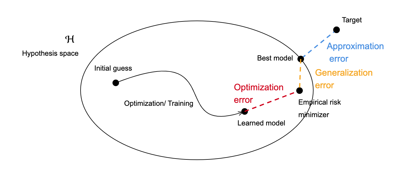 FIGURE 2. Diagram representing the learning procedure, the three main paradigms and their corresponding errors.
2 Shallow Neural Networks
We shall focus from now on on the first paradigm: the approximation of an objective function using a suitable parametric space. We introduce neural networks (NNs) as a class of hypothesis spaces whose name and structure are inspired by the human brain. They where first developed as an attempt to mathematically model the way in which biological neurons interact with each other through electrical nerve signals. It is clear that such models are oversimplified with respect to the complex human physiology, but they still form a class of powerful machine learning models showing
unique properties.
The simplest form of neural networks are called Shallow Neural Networks (SNNs), which are defined as the following parametric hypothesis space:
\mathcal{H} =\left\{F_M:\mathbb{R}\rightarrow\mathbb{R}\left|\right.F_M(\mathbf{x}) =\sum_{i=1}^{M}w_i\sigma(\mathbf{a_i}^T\cdot \mathbf{x}+b_i),\;w_i\in\mathbb{R},\mathbf{a_i}\in\mathbb{R}^d,b_i\in\mathbb{R}, M\in\mathbb{N}\right\},
where \sigma:\mathbb{R}\rightarrow\mathbb{R} is called the activation function and has a nonlinear form that gives the SNN its fine approximating properties. Some common choices for \sigma include
\text{ReLU: } \sigma(z)=\max(0,z),\qquad \sigma(z)=\tanh(z),\qquad \sigma(z)=\frac{1}{1+\exp{-z}}).
The ReLU activation function is generally the most common choice, and we will focus on it throughout this post. The parameters w_i are referred to as weights, while the other parameters a_i and b_i are respectively called the coefficients and the biases. Finally, the index M is the width of the SNN and controls the complexity of the model. To mention,
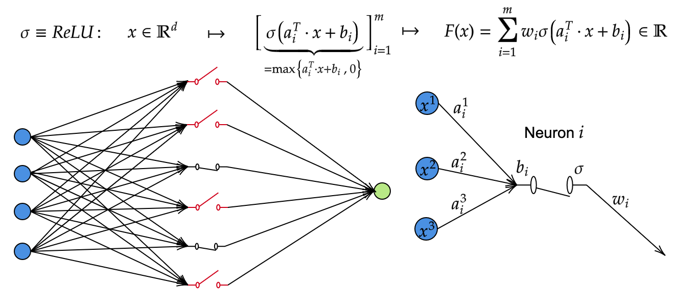 FIGURE 3. On the left, representation of a SNN as a network composed of several interconnected simple units called neurons distributed in three layers: (from left to right) the input layer, the hidden layer and the output layer (from left to right). On the right, diagram showing the operations that take place on each particular neuron.
There are more complex classes of neural networks. Deep Neural Networks (DNNs) refer to those which are constructed as the composition of several simple architectures, like SNNs, by increasing their number of hidden layers, that we call the depth of the model. Two of the most popular choices are:
• Multilayer Perceptron (MLP) of depth K:
\mathcal{H}_K=\left\{F_K:F_K(\mathbf{x})=\mathbf{w^T}\mathbf{x}(K),\;\mathbf{w}\in\mathbb{R}^{d_K} \right\}
being x(K) the final point of the discrete dynamical system given by
\mathbf{x}(k+1)=\mathbf{w}(k)\sigma\left(\mathbf{a}(k)^T\mathbf{x}(k)+b(k)\right), x(0) = x, for k = 0, . . . , K − 1, where \qquad \mathbf{w}(k)\in\mathbb{R}^{d_{k+1}},\qquad \mathbf{a}(k)\in\mathbb{R}^{d_k},\qquad b(k)\in\mathbb{R},
and d_0 = d, d_k \in\mathbb{N} for all
• Residual Neural Networks, obtained by redefining the dynamical system of the MLP as
\mathbf{x}(k+1)=\mathbf{x}(k) + \mathbf{w(k)}\sigma \left(\mathbf{a}(k)^T\mathbf{x}(k)+b(k)\right).
2.1 Approximation properties
As mentioned above, neural networks have a number of very interesting properties for function approximation. In particular, and despite their apparent simplicity, the architecture of SNNs is sufficient to prove some very strong approximation results. One of the most classical ones is the Universal Approximation Theorem, proven by Cybenko in 1989 (see [4]), where the space of functions to be approximated is taken as the space of continuous functions in a compact set of \mathbb{R}^d with the topology of uniform convergence:
Theorem 2.1
Let \Omega\subset\mathbb{R}^d be a compact set, and F^*\in C(\Omega). Assume that the activation function \sigma is continuous and sigmoidal, i.e. \lim_{z\rightarrow\infty}\sigma(z)=1, \lim_{z\rightarrow-\infty}\sigma(z)=0. Then, for every \epsilon>0 there exists F_M\in\mathcal{H} such that
\|F_M-F^*\|_{C(\Omega)}=\max_{\mathbf{x}\in \Omega}|F_M(\mathbf{x})-F^*(\mathbf{x})| \lt \epsilon. \qquad (1)
The proof follows from an application of the Hahn-Banach theorem and the Riesz-Markov representation theorem, together with an argument based on the non-degenerate properties of \sigma.
It can be easily seen that the activation function ReLU does not verify the hypotheses of the theorem as it is not bounded. Fortunately, different versions and generalizations of the above result have been proven. Here we show the following universal approximation theorem of Pinkus ([6]), which is striking for the equivalence it establishes:
Theorem 2.2
Let \Omega\subset\mathbb{R}^d be a compact set and \sigma a continuous activation function. Then, \mathcal{H} is dense in C(\Omega) in the topology of uniform convergence if and only if \sigma is non-polynomial.
2.2 Curse of dimensionality
Now that we know that a continuous function defined on a compact set can be approximated by an SNN with an arbitrarily small error (and thus, any measurable function too, due to Lusin’s Theorem), one may mistakenly think that this is already sufficient to ensure the existence of methods that converge to a continuous objective function in a feasible way.
It turns out that this is not true: there is a type of difficulties that arise when working with high-dimensional data which people refer to as the “curse of dimensionality”. They usually express the difficulties and enormous increase in the computational efforts required for the processing and analysis of a dataset due to mathematical phenomena like the concentration of distances, but also caused by the explosive tendencies of certain functions or parameters when the dimension of the input space increases.
In our case, the curse of dimensionality is exhibited on the complexity of our SNN (i.e., its width M), which depends exponentially dependence on the dimension of the input space in the expression of the approximation error bound in L^p norm:
\|F_M-F^*\|_{L^p(\Omega)}\leq C \frac{\|F^*\|_{W^{s,p}(\Omega)}}{M^{\alpha(s)/d}}, \qquad(2)
being C>0 a constant that depends on \Omega and the Sobolev parameters (s,p). From (2), it follows that we need a width of M\gtrsim\epsilon^{d\alpha} to obtain an approximation error of \epsilon, meaning that the complexity of the necessary approximation SNN becomes enormous in high dimensions.
Several approaches can be taken to overcome this difficulty, but the most basic one is to consider a smaller set of problems until we identify the functions that require a complexity whose dependence with d for fixed \epsilon is at most polynomial: it is a matter of finding the “right” space of functions to approximate.
This correspondence of an approximation method with a space of functions where the algorithm is well suited a clear analog in classical numerical analysis. Finite element methods and splines are two schemes that use piecewise polynomials to approximate a particular function that usually lies in a particular Sobolev or Besov space.
It turns that those two classes of spaces are the “right” ones for this approximation problem because the functions that motivate the problem are solutions of PDEs that lie on them, but also due to the existence of direct and inverse approximation theorems. Roughly speaking, a function can be approximated by piecewise polynomials with certain convergence rate if and only if it lies in a certain Sobolev or Besov space.
Barron spaces
Barron spaces are constructed by trying to mimic the mentioned approach and find the functions that can be approximated by “well-behaved” two-layer neural networks.
Let \Omega\in\mathbb{R}^d be a compact set and \sigma\equivReLU. We consider the functions f:\Omega\rightarrow\mathbb{R} that admit the representation
f(\mathbf{x})=\int_{\Theta}w\sigma(\mathbf{a}^T\mathbf{x}+c)\rho(dw,\mathbf{da},db)=\mathbb{E}_\rho[w\sigma(\mathbf{a}^T\mathbf{x}+b)],\qquad \mathbf{x}\in\Omega, \qquad (3)
where \Theta=\mathbb{R}\times\mathbb{R}^d\times\mathbb{R} space of parameters and \rho is a probability distribution on (\Theta,\Sigma_\Theta), being \Sigma_\Theta a Borel \sigma-algebra on \Theta. We can intuitively think of \rho as an hypothetical unknown probability distribution of the parameters that is the limit to which converges the sum of atomic measures defined by the specific finite set of parameters of a DNN when its width (or, equivalently, the number of parameter samples) tends to infinity. With the expression (3), approximating F^* with a SNN becomes a Montecarlo integration problem.
This interpretation is depicted in the picture below.
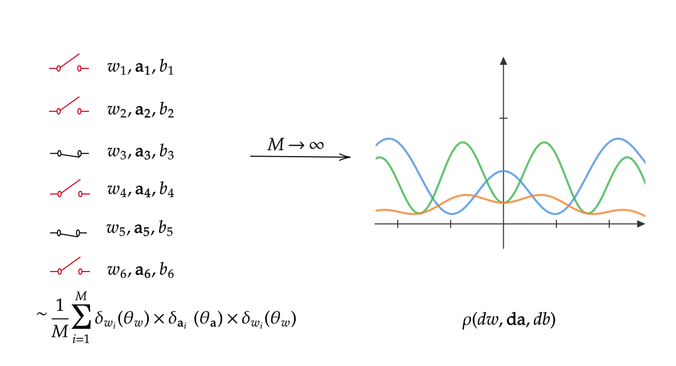
FIGURE 4. Diagram representing the probability distribution ρ on the space of parameters as the continuum width analog of SNNs.
In general, the measure \rho for which the representation (3) holds is not unique. For a function that admits this representation, we define for 1\leq p\leq\infty its p-Barron norm \|\cdot\|_{\mathcal{B}_p} as
\|f\|_{\mathcal{B}_p}=\inf_\rho\left(\mathbb{E}_\rho[|w|^p(\|\mathbf{a}\|_1+|b|)^p]\right)^{1/p},\qquad 1\leq p\leq\infty, \qquad (4)
where the infimum is taken over all \rho for which (3) holds for all \mathbf{x}\in\Omega. Now, for 1\leq p\leq\infty, the p-Barron space \mathcal{B}_p is defined as
\{f\in C(\Omega): f \text{ admits a representation }(3), \|f\|_{\mathcal{B}_p} \lt \infty\}.
Note that, by Hölder’s inequality, it is straightforward that
\mathcal{B}_\infty\subset\cdots\subset\mathcal{B}_2\subset\mathcal{B}_1.
To see this, given p\leq q, we have that, for all f\in C(\Omega),
\left(\int_\Theta|a|^pd\rho\right)^{1/p}\leq\left(\int_\Theta|a|^qd\rho\right)^{1/q}\left(\int_\Theta d\rho\right)^{\frac{q-p}{q}}\Rightarrow \|f\|_{\mathcal{B}_p}\leq\|f\|_{\mathcal{B}_q}.
The opposite inclusions are also true (see [1]):
Proposition 1
For any f\in \mathcal{B}_1, we have f\in \mathcal{B}_\infty and
\|f\|_{\mathcal{B}_1}=\|f\|_{\mathcal{B}_\infty}.
As a consequence, we have that for any 1\leq p \lt \infty, \mathcal{B}_p=\mathcal{B}_\infty and \|f\|_{\mathcal{B}_p}=\|f\|_{\mathcal{B}_\infty}, this is, there is just one Barron space and one Barron norm that we denote by \mathcal{B} and \|\cdot\|_\mathcal{B}, respectively.
Having defined the Barron space, it is natural to think what kind of functions belong to it. To answer this question, it is necessary to refer to Barron’s seminal paper of 1993 [1], in which he showed that functions verifying an spectral regularity property would improve the approximation bound by SNNs in L^2 helping to partially overcome the curse of dimensionality.
Before stating an extended version of its main result (proven in [2]), we recall one basic definition in harmonic analysis:
The Fourier transform of a function f:\mathbb{R}^d\rightarrow\mathbb{R} is
\hat f(\xi)=\frac{1}{(2\pi)^d}\int_{\mathbb{R}^d}f(\mathbf{x})e^{-i\xi\cdot \mathbf{x}}\mathbf{dx}.
and verifies the property \widehat{Df}(\xi)=i\xi\hat f(\xi), which means it transforms derivatives in products.
Theorem 3.1
For a function F^*:\Omega\rightarrow\mathbb{R}, let \hat F^* be the Fourier transform of any extension of F^* to \mathbb{R}^d. If
\gamma(F^*):=\inf_{\hat F}\int_{\mathbb{R}^d}\|\xi\|_1^2|\hat F^*(\xi)|d\xi=\|\widehat{D^2 F^*}\|_1 \lt +\infty,
then for any M>0 there exists a SNN F_M(\mathbf{x})=\frac{1}{M}\sum_{i=1}^Mw_i\sigma(\mathbf{a_i}^T\mathbf{x}+b_i) satisfying
\|F_M-F^*\|_{L^2(\Omega)}^2\leq\frac{3\gamma(F^*)^2}{M},
and \frac{1}{M}\sum_{i=1}^M|w_i|(\|\mathbf{a_i}\|_1+|b_i|)\leq\frac{2\gamma(F^*)}{M}.
As we can see, the theorem states that the L^1-integrability of the Fourier transform of the second derivative of a function F^* is a sufficient condition to ensure the disappearance of the exponential dependence of the width M with the dimension in the error bound in norm L^2.
Note that the numerator \gamma(F^*) is an integral over \mathbb{R}^d and could therefore bring back to the bound an exponential dependence on dimension. This means that the finiteness of \gamma(F^*) if generally not enough to avoid the curse of dimensionality, but there are many examples for which \gamma(F^*) is only moderately large, e.g., O(d) or O(d^2), like gaussian functions.
On the second part of the result, we can see that a finite analog of the Barron norm for SNNs is also upper bounded by the coefficient \gamma(F^*). This weighted sum is defined as the path norm of the network,
\|\theta\|_\mathcal{P}:=\frac{1}{M}\sum_{i=1}^M|w_i|(\|\mathbf{a_i}\|_1+|b_i|),
where \theta denotes its correspondent set of parameters \{(w_i,\mathbf{a}_i,b_i)\}_{i=1}^M. As the analog of \|\cdot\|_\mathcal{B}, it is natural to consider two-layer neural networks with bounded path norm when studying their approximation properties.
The subsequent theorem finally sheds some light on a class of functions that belong to \mathcal{B}:
Theorem 3.2
Let F^*\in C(\Omega) and assume that F^* satisfies \gamma(F^*) \lt \infty. Then F^* admits an integral representation (3).
Moreover,
\|F^*\|_{\mathcal{B}}\leq2\gamma(F^*)+2\|\nabla F^*(0)\|_1+2|F^*(0)|.
A necessary condition for a function F* to verify that \gamma(F^*) \lt \infty is the boundedness of all its first order partial derivatives, which constitutes a big restriction for those functions. On the other hand, it is enough for a function to satify \gamma(F^*) if F^* has all partial derivatives of order less or equal than s in the space L^2(\mathbb{R}^d), being s=\lceil1+d/2\rceil.
By finiteness of \gamma(F^*), it is immediate the following result:
Corollary 1
All gaussian functions, positive definite functions, linear functions and radial functions belong to \mathcal{B}.
Having defined the Barron space and characterized some functions that belong to it, we state the two results, extracted from [5] and proven there, that identify this space as the appropriate one to be approximated by SNNs.
Theorem 3.3
(Theorem of direct approximation)
For any F^*\in\mathcal{B} and M>0, there exists a SNN F_M(\mathbf{x})=\frac{1}{M}\sum_{i=1}^Mw_i\sigma(\mathbf{a_i}^T\mathbf{x}+b_i) satisfying
\|F_M(\cdot;\theta)-F^*(\cdot)\|_{L^2(\Omega)}^2\leq\frac{3\|F^*\|^2_\mathcal{B}}{M}.
Furthermore, we have \|\theta\|_\mathcal{P}\leq2\|F^*\|_\mathcal{B}.
To state the reciprocal final result, which is very important as it states the characterization of \mathcal{B} as the right approximation function space with respect to the path norm, we define \mathcal{N}_Q:=\{F_M(\cdot;\theta):\;\|\theta\|_\mathcal{P}\leq Q,m\in\mathbb{N}^+\}.
Theorem 3.4
(Theorem of inverse approximation)
Let F^*\in C(\Omega). Assume there exists a constant Q and a sequence of functions (F_M)\subset\mathcal{N}_Q such that
\lim_{M\rightarrow\infty}F_M(\mathbf{x})= F^*(\mathbf{x}),
for all \mathbf{x}\in\Omega. Then F^*\in\mathcal{B} and \|F^*\|_\mathcal{B}\leq Q.
We give a brief idea of the proof:
Assume that F_M(\mathbf{x})=\frac{1}{M}\sum_{i=1}^Mw_i^{(M)}\sigma\left(\mathbf{a}_i^{(M)}\mathbf{x}+b_i^{(M)}\right). The theorem’s hypothesis implies that the sequence (\rho_M) defined by
\rho_M(w,\mathbf{a},b)=\frac{1}{M}\sum_{i=1}^M\delta(w-w_i^{(M)})\delta(\mathbf{a}-\mathbf{a}_i^{(M)})\delta(b-b_i^{(M)})
is tight. By Prokhorov’s Theorem, there exists a subsequence (\rho_{M_k}) and a probability measure \rho^* such that \rho_{M_k} converges weakly to \rho^*. This measure \rho^* on the parameter space \Theta is the one associated to F^* that makes it belong to \mathcal{B} with a Barron norm bounded by Q.
4 Conclusions and open questions
The Barron space \mathcal{B} catches all the functions that can be approximated by SNNs with bounded path norm, and the bound of the corresponding error partially overcomes the curse of dimensionality.
Due to the statement of the two theorems, \mathcal{B} can be seen as the closure of the space of DNNs \mathcal{H}_\Theta with respect to the path norm, which means it is the largest function space that is well approximated by SNNs, and the Barron norm is the natural norm associated to it. Target functions outside \mathcal{B} may be increasingly difficult to approximate by SNNs as dimension increases.
We end this post by listing three open paths for research on the subject:
1. More specific descriptions of the functions that belong to \mathcal{B}.
2. Further study on the possibilities and conditions for PDE solutions to lie on the Barron space (see [3]). The goal is the application of SNNs to approximate the solutions of high-dimensional PDEs.
3. Extension of this theory to more complex architectures like Deep Neural Networks. In the specific case of Residual Neural Networks, there is current research on this direction (see [5]).
\end{enumerate}
References
[1] A. Barron. “Universal approximation bounds for superpositions of a sigmoidal function”. In: IEEE Transactions on Information Theory 39.3 (1993), pp. 930– 945. doi: 10.1109/18.256500.
[2] L. Breiman. “Hinging hyperplanes for regression, classification, and function approximation”. In: IEEE Transactions on Information Theory 39.3 (1993), pp. 999–1013. doi: 10.1109/18.256506.
[3] Z. Chen, J. Lu, and Y. Lu. “On the representation of solutions to elliptic pdes in barron spaces”. In: Advances in neural information processing systems 34 (2021), pp. 6454–6465.
[4] G. Cybenko. “Approximation by superpositions of a sigmoidal function”. In: Mathematics of control, signals and systems 2.4 (1989), pp. 303–314.
[5] C. Ma, L. Wu, et al. “The Barron space and the flow-induced function spaces for neural network models”. In: Constructive Approximation 55.1 (2022), pp. 369– 406.
[6] A. Pinkus. “Approximation theory of the MLP model in neural networks”. In: Acta Numerica 8 (1999), pp. 143–195.
|| Go to the Math & Research main page


