Generalization bounds for neural ODEs: A user-friendly guide

Once a neural network is trained, how can one measure its performance on new, unseen data? This concept is known as generalization.

While many theoretical models exist, practical models often lack comprehensive generalization results. This post introduces a probabilistic approach to quantify the error of a model after training.

The problem

We are inspired by previous research ([1]) and consider a specific model defined as:

$x'(t) = W(t) \sigma\left(A(t)x(t) + b(t)\right), (1.1)$

where $W, A$ and $b$ are bounded functions.

This model is the continuous version of discrete-time ResNets:

$x_{k + 1} = x_k + W_k \sigma (A_k x_k + b_k).$

For a given input $x_0$ , solving equation (1.1) with $x(0) = x_0$ gives the model’s output as $x(1)$ .

Given a dataset $(x_i, y_i)_{i = 1, \cdots, n} \overset{\text{i.i.d.}}{\sim} \mu$ with independent and identically distributed (i.i.d.) samples from an unknown distribution $\mu$ , the model’s performance can be assessed using a loss function $\ell$ :

$\mathcal{R}(f) = \mathbb{E}_{(x, y) \sim \mu}\left[ \ell(y, f(x)) \right].$

In practice, the empirical risk is often considered instead:

$\displaystyle \widehat{\mathcal{R}}_n(f) = \frac1n \sum_{i = 1}^n \ell(y_i, f(x_i)).$

But how can we retrieve information on $\mathcal{R}(f)$ from the sole knowledge of $\widehat{\mathcal{R}}_n(f)$ ?

Generalization bounds consist in upper-bounding the difference between $\mathcal{R}(f)$ and $\widehat{\mathcal{R}}_n(f)$ .

Generalization bounds

We focus on neural ODEs defined by
$x'(t) = W(t) \sigma\left( A(t)x(t) + b(t) \right)$ for $t\in[0, 1]$ , where
$W: [0, 1] \to \mathbb{R}^{d\times p}, A: [0, 1] \to \mathbb{R}^{p\times d}, b: [0, 1] \to \mathbb{R}^{p}$ are bounded functions, and where $p$ is the width of the model.

The activation function $\sigma: \mathbb{R} \to \mathbb{R}$ is assumed to be $K_\sigma$ -Lipschitz and to satisfy $\sigma(0) = 0$ (e.g. ReLU: $x \mapsto \max(x, 0)$ or $\tanh$ , see Figure 1). The loss function $\ell$ is assumed to be $K_\ell$ -Lipschitz.

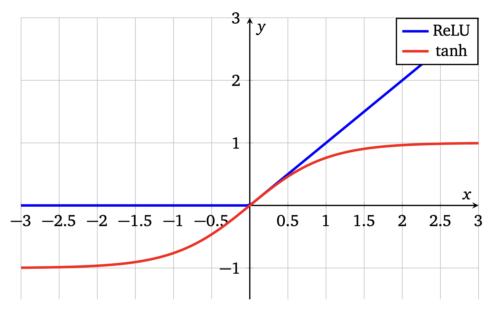
Figure 1. Examples of activation functions

To establish generalization bounds, we approximate any control $\theta$ within a finite set of controls. This approximation allows us to simplify the problem by focusing on a finite number of scenarios (see Figure 2).

Using piecewise constant controls, we ensure our functions jump at specific points, which aligns with the continuous nature of neural ODEs derived from discrete-time ResNets.

The idea of the proof is, for every $\varepsilon > 0$ , to find a finite number of controls $\theta_1, \cdots, \theta_{\mathcal{N}(\varepsilon)}$ such that $\forall\theta\in\Theta, \exists i \in \left\{ 1, \cdots, \mathcal{N}(\varepsilon) \right\}, \| \theta - \theta_i \| \leq \varepsilon$ .

Why? Because under our assumptions, one can prove that both $\mathcal{R}$ and $\widehat{\mathcal{R}}_n$ are $C$ -Lipschitz for some $C > 0$ . Then for every $\theta\in\Theta$ , if $\| \theta - \theta_i \| \leq \varepsilon$ ,

$\begin{aligned} \left| \mathcal{R}(\theta) - \widehat{\mathcal{R}}_n(\theta) \right| & \leq \left| \mathcal{R}(\theta) - \mathcal{R}(\theta_i) \right| + \left| \mathcal{R}(\theta_i) - \widehat{\mathcal{R}}_n(\theta_i) \right| + \left| \widehat{\mathcal{R}}_n(\theta_i) - \widehat{\mathcal{R}}_n(\theta) \right| \\ & \leq 2C\varepsilon + \underset{j \in \{ 1, \cdots, \mathcal{N}(\varepsilon) \}}{\max} \left| \mathcal{R}(\theta_j) - \widehat{\mathcal{R}}_n(\theta_j) \right|. \end{aligned}$

So instead of upper-bounding

$\left| \mathcal{R}(\theta) - \widehat{\mathcal{R}}_n(\theta) \right|$

for every $\theta\in\Theta$ , one can do it only for a finite number of them.

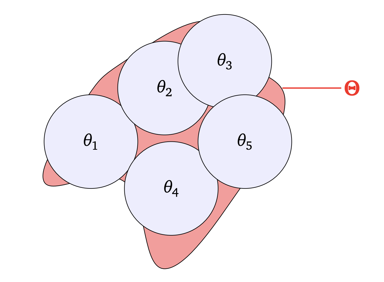
Figure 2. An almost cover of $Theta$

Obviously if $W, A, b$ are only assumed to be bounded, we will not be able to find a finite covering number.

Instead, we restrict ourselves to piecewise constant controls, motivated by interpolation results for such neural ODEs as in [2]. However, even then, the covering number is infinite: for a piecewise constant function to be well approximated by other piecewise constant functions, these other functions must jump at the same points (see Figure 3).

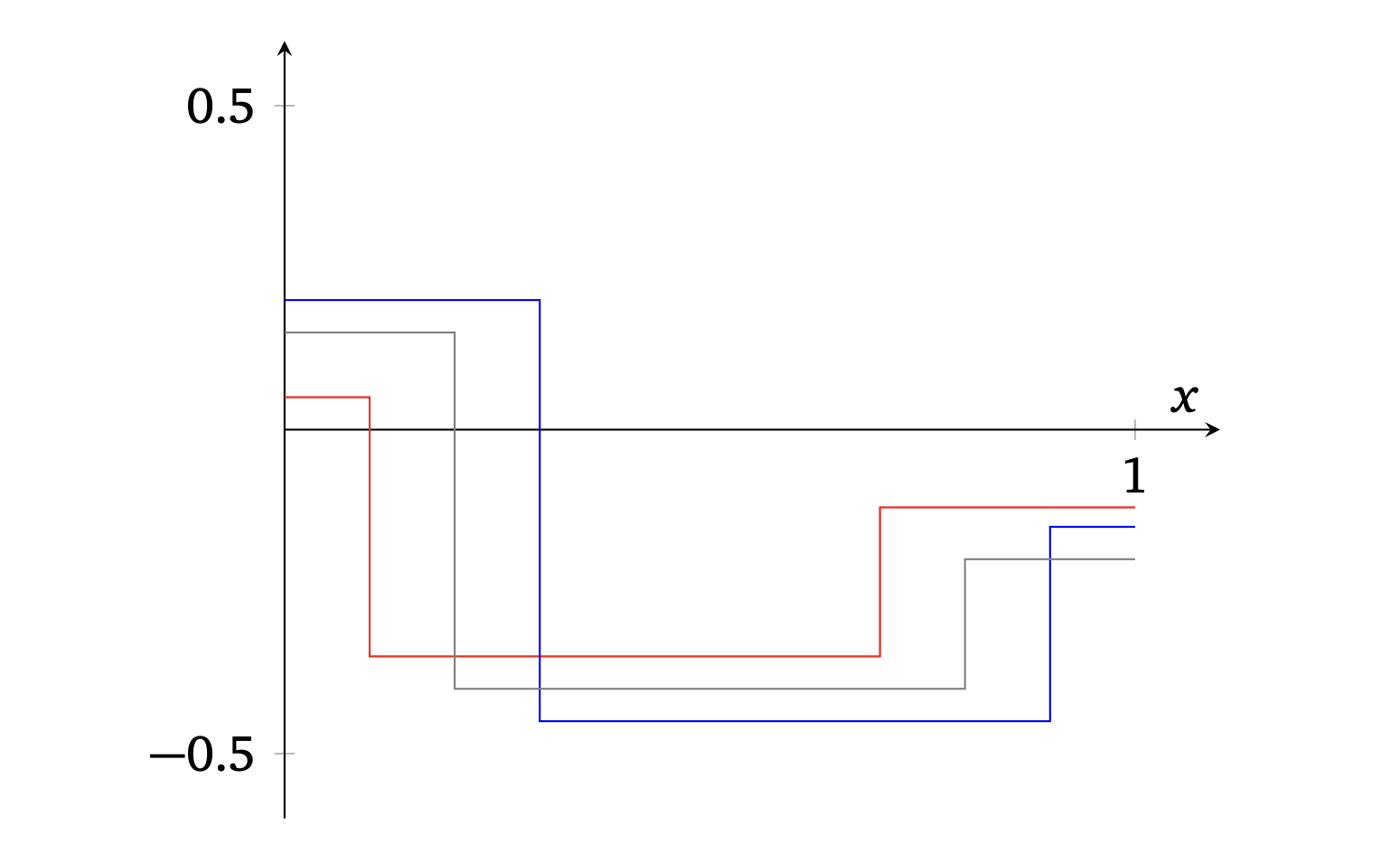
Figure 3. For the red and blue functions to approximate the gray one, they need to jump for the same values of $x$

So we decide to restrict ourselves to piecewise constant controls, with jumps at specific times, e.g. $\left\{ \dfrac1r, \dfrac2r, \dots, \dfrac{r-1}{r} \right\}$ for some integer $r \geq 1$ .

This is reasonable considering the fact that the neural ODE we consider is the continuous version of a discrete-time ResNet, with jumps in discrete time.

If we set

$E := L^\infty \left( (0, 1), \mathbb{R}^{d \times p} \times \mathbb{R}^{p \times d} \times \mathbb{R}^{p} \right),$

our set of controls is then:

$\Theta = \left\{ \theta = (W, A, b) \in E \mid \| \theta \|_{\infty, 1, \infty} \leq R_\Theta, \text{ piecewise constant with only jumps at } \dfrac{k}{r}, k \in \{ 1, \cdots, r - 1 \} \right\},$

where for

$\theta=(W,A,b)\in E,$

$\| \theta \|_{\infty, 1, \infty} := \max\left( \sum_{i = 1}^p \| w_i \|_\infty, \sum_{i = 1}^p \| a_i \|_\infty, \sum_{i = 1}^p \| b_i \|_\infty \right).$

Then, one can show the following upper-bound on the covering number:

Lemma 2.1
For $\varepsilon > 0$ , let $\mathcal{N}(\varepsilon)$ be the $\varepsilon$ -covering number of $\Theta$ for the norm $\| \cdot \|_{\infty, 1, \infty}$ . Then

$\log \mathcal{N}(\varepsilon) \leq p (2d + 1) r \log\left( \dfrac{2p R_\Theta}{\varepsilon} \right).$

Then we can establish a generalization bound:

Proposition 2.2
If $n \geq (pR_\Theta)^{-2}$ , $R_\Theta \geq 1$ , $R_{\mathcal{Y}} \geq 1$ then with probability at least $1 - \delta$ ,

$\forall \theta \in \Theta, \left| \mathcal{R}(\theta) - \widehat{\mathcal{R}}_n(\theta) \right| \leq \frac{2BK_\sigma}{\sqrt{n}} + \frac{B}{2} \sqrt{\frac{2 \left( p (2d + 1) r + 1 \right) \log\left( 2 p R_\Theta \sqrt{n} \right)}{n}} + \frac{B}{\sqrt{2n}} \sqrt{\log\frac{1}{\delta}},$

where

$B = 2 K_{\ell} R_\Theta \left(R_{\mathcal{X}} + R_{\mathcal{Y}} + K_\sigma R_\Theta^2 \left(1 + R_{\mathcal{X}}\right) \exp\left( K_\sigma \left(R_\Theta \right)^2 \right) \right) \exp\left(K_\sigma R_\Theta^2 \right).$

Idea of the proof
The first step consists in controlling the trajectories using Grönwall’s inequality: there exists $M > 0$ such that $\forall x \in \mathcal{X}, \forall\theta\in\Theta, \| F_\theta(x) \| \leq M$ , from which we deduce there exists $\overline{M} > 0$ such that $\forall x \in \mathcal{X}, \forall y \in \mathcal{Y}, \forall\theta\in\Theta, \left| \ell\left(F_\theta(x), y\right) \right| \leq \overline{M}$ .

Using this remark, McDiarmid’s inequality and the remark we made earlier, we obtain that with probability at least $1 - \delta$ , for each $\theta\in\Theta$ ,

$\left| \mathcal{R}(\theta) - \widehat{\mathcal{R}}_n(\theta) \right| \leq \mathbb{E}\left[ \underset{\theta' \in \Theta}{\sup} \left| \mathcal{R}(\theta') - \widehat{\mathcal{R}}_n(\theta') \right| \right] + \frac{\overline{M}\sqrt{2}}{\sqrt{n}} \sqrt{\log\frac{1}{\delta}} \\ \leq 2C\varepsilon + \mathbb{E}\left[ \underset{j \in \{ 1, \cdots, \mathcal{N}(\varepsilon) \}}{\max} \left| \mathcal{R}(\theta_j) - \widehat{\mathcal{R}}_n(\theta_j) \right| \right] + \frac{\overline{M}\sqrt{2}}{\sqrt{n}} \sqrt{\log\frac{1}{\delta}}$

To conclude, we use the fact that for each $j$ , the random variable $\widehat{\mathcal{R}}_n(\theta_j)$ is $\dfrac{\overline{M}^2}{n}$ -subgaussian, with expected value
$\mathcal{R}(\theta_j)$ , and some basic computations then lead to the above Proposition.

Numerical results

A question that arises is whether the bound from Proposition 2.2, or its corollaries, can be applied in practice.

The fact is that this will highly depend on the settings. Indeed, the number $B$ tends to be quickly very large, especially because of the presence of the exponential function. However, if $n$ is large enough, then compensations happen, which may lead to a useful upper-bound.

Note that when $R_\Theta$ is large, the model is more complex, and may thus learn more complex tasks, yielding a higher value of $\widehat{\mathcal{R}}_n(\theta)$ . But this also leads to a higher value for $B$ , and therefore to a larger upper-bound for $\left| \mathcal{R}(\theta) - \widehat{\mathcal{R}}_n(\theta) \right|$ . So for the bound to be interesting, $R_\Theta$ must not be too low, but it must not be too large either, and the same holds for $p$ and $r$ . However, if $n$ is large enough, then it may compensate all the previous effects.

To test these bounds, consider a $2D$ binary classification task, with $n = 10,000$ training points.

By applying the derived bounds, we calculate the probability of the model being wrong. As shown in Figure 4, the bounds provide insights into the model’s performance on unseen data.

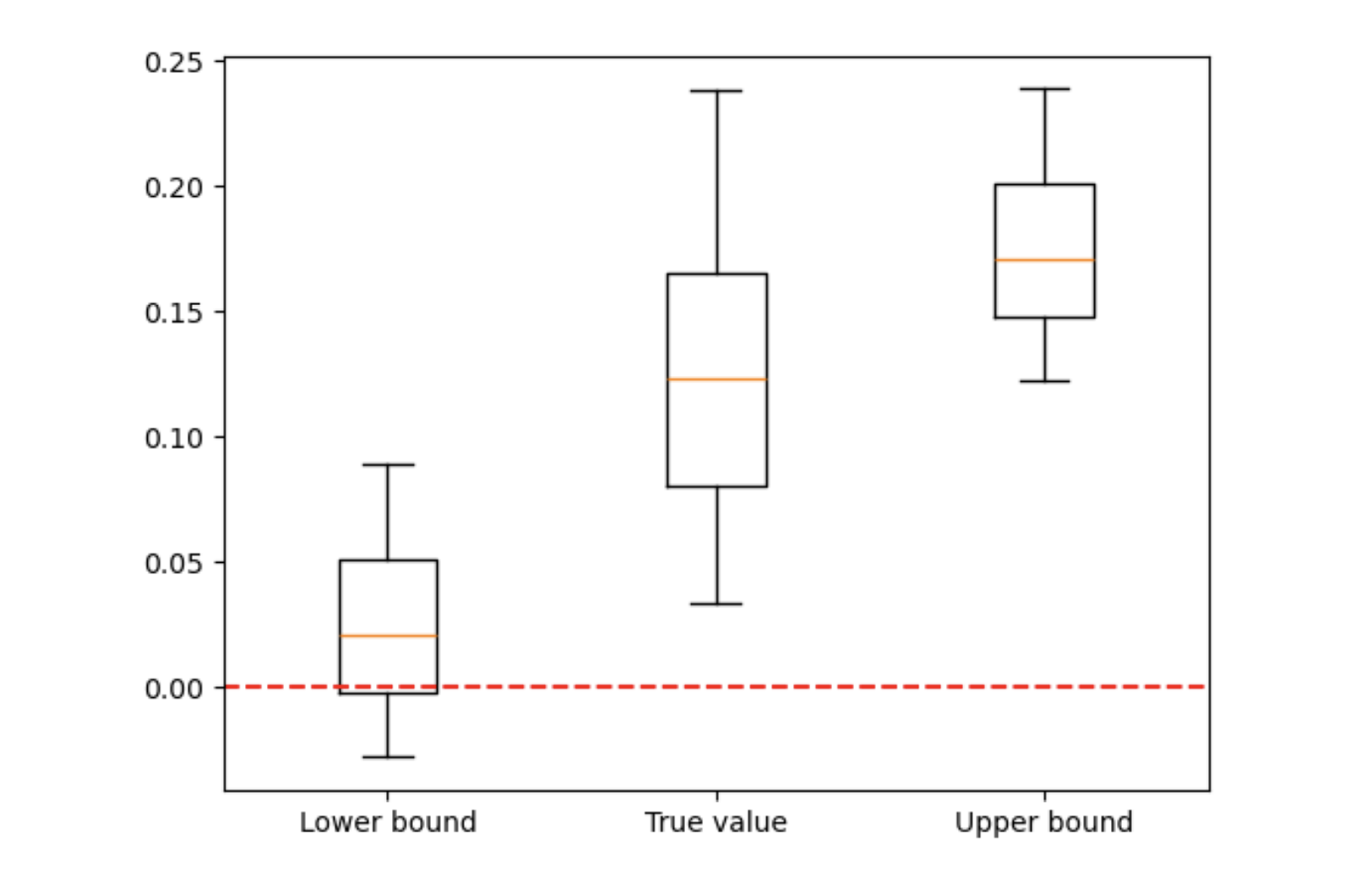
Figure 4. Generalization bounds

We see that the lower-bound can be negative, when the true value obviously cannot.

Future work

This post establishes generalization bounds for neural ODEs, demonstrating their learning capability.
These bounds are of little practical use, but show, when combined with interpolation results such as in [2].
that such models can indeed learn.

Future research could develop more practical bounds using specific training algorithms.

References

[1] P. Marion (2024) Generalization bounds for neural ordinary differential equations and deep residual networks. Advances in Neural Information Processing Systems. Vol. 36.
[2] A. Alvarez-Lopez, A. H. Slimane, E. Zuazua (2024) Interplay between depth and width for interpolation in neural ODEs. arXiv preprint arXiv:2401.09902