
Stochastic optimization for simultaneous control
Umberto Biccari, DeustoCCM
What is a simultaneous control problem?
Consider the following parameter-dependent linear control system
\begin{cases} x'_\nu(t) = A_\nu x_\nu(t)+B u(t), & 0<t<T, \\ x_\nu(0) = x^0, \end{cases}
with
\mathbf{A}_\nu=\left(\begin{array}{cccccc} 0 & 1 & 0 & \ldots & \ldots & 0 \\ 0 & 0 & 1 & 0 & \ldots & 0 \\ \vdots & & & \ddots & \ddots & \vdots \\ 0 & \ldots & \ldots & \ldots & 1 & 0 \\ -\nu & 0 & \ldots & \ldots & \ldots & 0 \end{array}\right)\in \R^{N\times N}, \quad B = \left(\begin{array}{c} 1 \\ 1 \\ \vdots \\ \vdots \\ 1\end{array}\right)\in \R^{N}.
The matrix \mathbf{A}_\nu is associated with the Brunovsky canonical form of the linear ODE
x^{(N)}_\nu(t) + \nu x_\nu(t) = 0,
where x^{(N)}_\nu(t) denotes the N-th derivative of the function x(t).
In (1)-(2), x_\nu(t)\in L^2(0,T;\R^N), N\geq 1, denotes the state, the N\times N matrix \mathbf{A}_\nu describes the dynamics, and the function u(t)\in L^2(0,T;\mathbb{R}^M), 1\leq M\leq N, is the M-component control acting on the system through the N\times M matrix \mathbf{B}. Here \nu\in \{\nu_1,\nu_2,\ldots,\nu_{|\mathcal K|}\}=:\mathcal K is a random parameter following a probability law \mu, with (\mathcal K,\mathcal F,\mu) the corresponding complete probability space.
With simultaneous controllability we refer to the problem of designing a unique parameter-independent control function capable to steer all the different realizations of (1) to some prescribed final target in time T, that is (see Figures 1 and 2):
x_\nu(T)=x^T\in\mathbb{R}^N, \quad \nu\in \mathcal{K} \;\;\;\;\mu-\text{a. e.}
How can we solve a simultaneous controllability problem?
The computation of a simultaneous control for (1)-(2) can be carried out through a standard optimal control methodology by solving the following minimization problem
\widehat{u}=\min_{u\in L^2(0,T;\R^M)} F_{\nu}(u) \\ F_{\nu}(u):= \frac{1}{2} \mathbb{E}\left[||{x_\nu(T)-x^T}||{\R^N}^2\right]+\frac{\beta}{2}||{u}||{L^2(0,T;\R^M)},
subject to the dynamics given by \eqref{linearsystem}. Here $\mathbb{E}[\cdot]$ denotes the expectation operator.
Typical approaches to solve the optimization problem (3) are (see [3]):
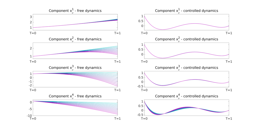 Figure 1. Evolution of the free (left) and controlled (right) dynamics of (2) with N = 4
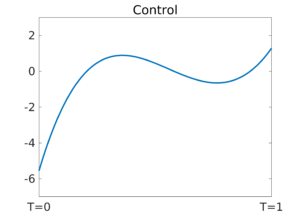 Figure 2. Parameter-independent control function associated to the plots in Figure 1
• The Gradient Descent (GD) algorithm: we find the minimizer \widehat{u} as the limit k\to +\infty of the following iterative process
\textbf{GD:} \quad u^{k+1} = u^k-\eta_k \left(\beta u^k - \frac{1}{|\mathcal K|}\sum_{\nu\in\mathcal K}B^\top p_\nu^k\right),where for all \nu\in\mathcal K the pair (x_\nu,p_\nu) solves the coupled system
\begin{cases} x'_\nu(t) = \mathbf{A}_\nu x_\nu(t)+\mathbf{B}u, & 0<t<T, \\ p'_\nu(t) = -\mathbf{A}_\nu^\top p_\nu(t), & 0<t<T, \\ x_\nu(0) = x^0, \quad p_\nu(T) = -(x_\nu(T)-x^T). \end{cases}
• The Conjugate Gradient (CG) algorithm: the gradient \nabla F_\nu is rewritten in the form
\nabla F_\nu(u) = \underbrace{(\beta I + \mathbb{E}[\mathcal L_{T,\nu}^\ast\mathcal L_{T,\nu}])}_{\mathbb{A}}u + \underbrace{\mathbb{E}[\mathcal L_{T,\nu}^\ast(y_\nu(T)-x^T)]}_{-b},where the operators \mathcal L_{T,\nu} and \mathcal L_{T,\nu}^\ast are defined as
\begin{array}{cccc} \mathcal L_{T,\nu}: & U &\longrightarrow &\mathbb{R}^N \\ & u & \longmapsto & z_\nu(T) \end{array} \quad \text{ and } \quad \begin{array}{cccc} \mathcal L_{T,\nu}^\ast: & \mathbb{R}^N &\longrightarrow & U \\ & p_{T,\nu} & \longmapsto & B^\top p_\nu, \end{array}with U:=L^2(0,T;\mathbb{R}^M) and
\begin{cases} y'_\nu(t) = \mathbf{A}_\nu y_\nu(t), & 0<t<T, \\ y_\nu(0) = x_0 \end{cases}and
\begin{cases} z'_\nu(t) = \mathbf{A}_\nu z_\nu(t) +\mathbf{B} u(t), & 0<t<T, \\ z_\nu(0) = 0. \end{cases}
We then use the conjugate gradient algorithm to solve the linear system \mathbb{A}u = b.
These two procedures are impractical when the cardinality of the parameter set \mathcal K is large because they require repeated resolutions of the dynamics (4) for all \nu\in \mathcal K.
This issue can be bypassed by employing a stochastic optimization method. In particular, we can consider the following approaches:
• Stochastic Gradient Descent (SGD) algorithm (see [2]): it is a drastic simplification of the classical GD in which, instead of computing the gradient of the functional for all parameters \nu\in\mathcal K, in each iteration this gradient is estimated on the basis of a single randomly picked configuration. This translates in the following recursion process
\textbf{SGD:} \quad u^{k+1} = u^k-\eta_k \left(\beta u^k - B^\top p_{\nu_k}^k\right).with \nu_k selected i.i.d. from \mathcal K.
• Continuous Stochastic Gradient (CSG) algorithm: it is a variant of SGD, based on the idea of reusing previously obtained information to improve the efficiency. The CSG recursion process for optimizing F_\nu is given by
\textbf{CSG:} \quad u^{k+1} = u^k-\eta_k \sum_{\ell = 1}^k \alpha_\ell\left(\beta u^\ell - B^\top p_{\nu_\ell}^\ell\right).where the weights \{\alpha_\ell\}_{\ell = 1}^k are obtained through the methodology presented in [4].
Experimental Results: comparison of the algorithms
We can test the efficiency of each one of the four aforementioned algorithms by performing simulations for increasing values of |\mathcal K|. In these simulations, we have chosen the initial state x^0 =(1,1,1,1)^\top and the final target x^T=(0,0,0,0)^\top. The time horizon is set to be T=1s. The parameter set is a |\mathcal K| points partition of the interval [1,6]: \mathcal K=\{\nu_1,\ldots,\nu_{|\mathcal K|}\} with \nu_1=1 and \nu_{|\mathcal K|}=6.
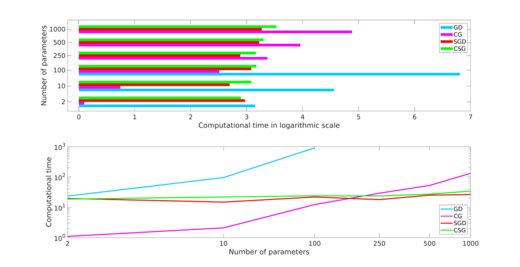
Figure 3 displays the computational times (in logarithmic scale) the four algorithms need to compute a simultaneous control for (1)-(2).
We can observe the following facts:
1. The GD algorithm is the one showing the worst performances. This because it has to copy with a high per-iteration cost but also with the fact that controllability problems are typically bad conditioned.
2. The CG algorithm is the one requiring the lower number of iterations to converge. This implies that CG is the best approach among the one considered when dealing with a low and moderate amount of parameters.
3. The stochastic approaches SGD and CSG appear to be insensitive to the cardinality of the parameter set. This fact is not surprising if we consider that, no matter how many parameters enter in our control problem, with SGD and CSG each iteration of the optimization process always requires only one resolution of the coupled system (4).
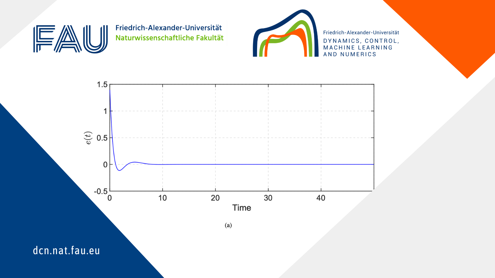
4. The CSG algorithm always outperforms SGD in terms of the number of iterations it requires to converge and, consequently, of the total computational time. This because in CSG the approximated gradient is close to the full gradient \nabla F_\nu of the objective functional when k\to +\infty. This translates in a less noisy optimization process with better convergence behavior (see Figure 4).
All these considerations corroborate the fact that, when dealing with large parameter sets, a stochastic approach is preferable to a deterministic one to address the simultaneous controllability of (1)-(2). A more complete discussion on the employment of stochastic optimization algorithms for simultaneous controllability can be found in [1].
 Figure 3. Computational time (in logarithmic scale) to converge to the tolerance \varepsilon = 10^{-4} of the GD, CG, SGD and CSG algorithms applied to the problem (2) with different values of |\mathcal K|.
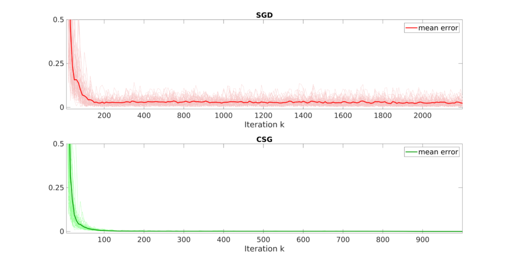 Figure 4. Convergence of the error for SGD and CSG. The plots correspond to 50 launches of the two algorithms with a tolerance \varepsilon = 10^{-4}.
References
[1] U. Biccari, A. Navarro-Quiles and E. Zuazua, Stochastic optimization methods for the simultaneous controllability of parameter-dependent systems, in preparation
|| Go to the Math & Research main page


