Hybrid parabolic-hyperbolic effect for heat equations with memory

Hybrid parabolic-hyperbolic effect for heat equations with memory

 

1 Introduction

PDEs with memory involve the past values of solutions. In the modeling, one physical quantity induces time-delayed actions on others, and and a large number of such actions form memory (as a time integral).

Such models with memory are far from being well understood. We need to develop mathematical methods to investigate new phenomena in the models, and then apply these methods to control problems.

 

2 Heat equations with memory in lower order terms

We begin with the following case that the memory is in the lower order term. Let \Omega\subset\mathbb R^n be a bounded domain (with a C^2-boundary). Define

A f := -\Delta f, \;\;\text{with its domain}\;\; D(A):=H^2(\Omega)\cap H_0^1(\Omega).

Write y(\cdot;y_0) for the solution of the following heat equation with memory:

\begin{cases} y^\prime(t) + A y(t) + \displaystyle\int_0^t M(t-s) y(s)ds = 0, ~t>0,\\ y(0)=y_0\in L^2(\Omega). \end{cases}

Formally, the model is heat + integral-type perturbation.

 

3 Hybrid parabolic-hyperbolic effect

(See [1]) Let N\geq 2 be an integer. Each solution y(\cdot;y_0) with y_0 \in L^2(\Omega) has the following decomposition:

y(t;y_0)= \textcolor{red}{ y_p(t;y_0) } + \textcolor{blue}{y_h(t;y_0) } + \text{remainder}, \hspace{0.5cm} t \geq 0.

where y_h and y_p are defined with explicit coefficients (p_l)_{l\geq 1} and (h_l)_{l\geq 1} (h_1 = - M):

\begin{cases} y_p(t;y_0) :=& e^{-tA}y_0 + \sum_{l=0}^{N-1} p_{l}(t) A^{-l-1} e^{-tA} y_0,\\ y_h(t;y_0) :=& \sum_{l=1}^{N-1} h_{l}(t) A^{-l-1} y_0 . \end{cases}

Moreover,

\sum_{l\geq 1} |p_l(t)| >0 ~~\text{and}~~ \sum_{l\geq 1} |h_l(t)|>0 ~~\text{for each}~~ t\geq 0.

In the above decomposition, we have the following:
• the parabolic component y_p(t;y_0) \in \displaystyle\bigcap_{k\in \mathbb N} D(A^k) for each t>0 (the infinite-order smoothing effect at positive time);

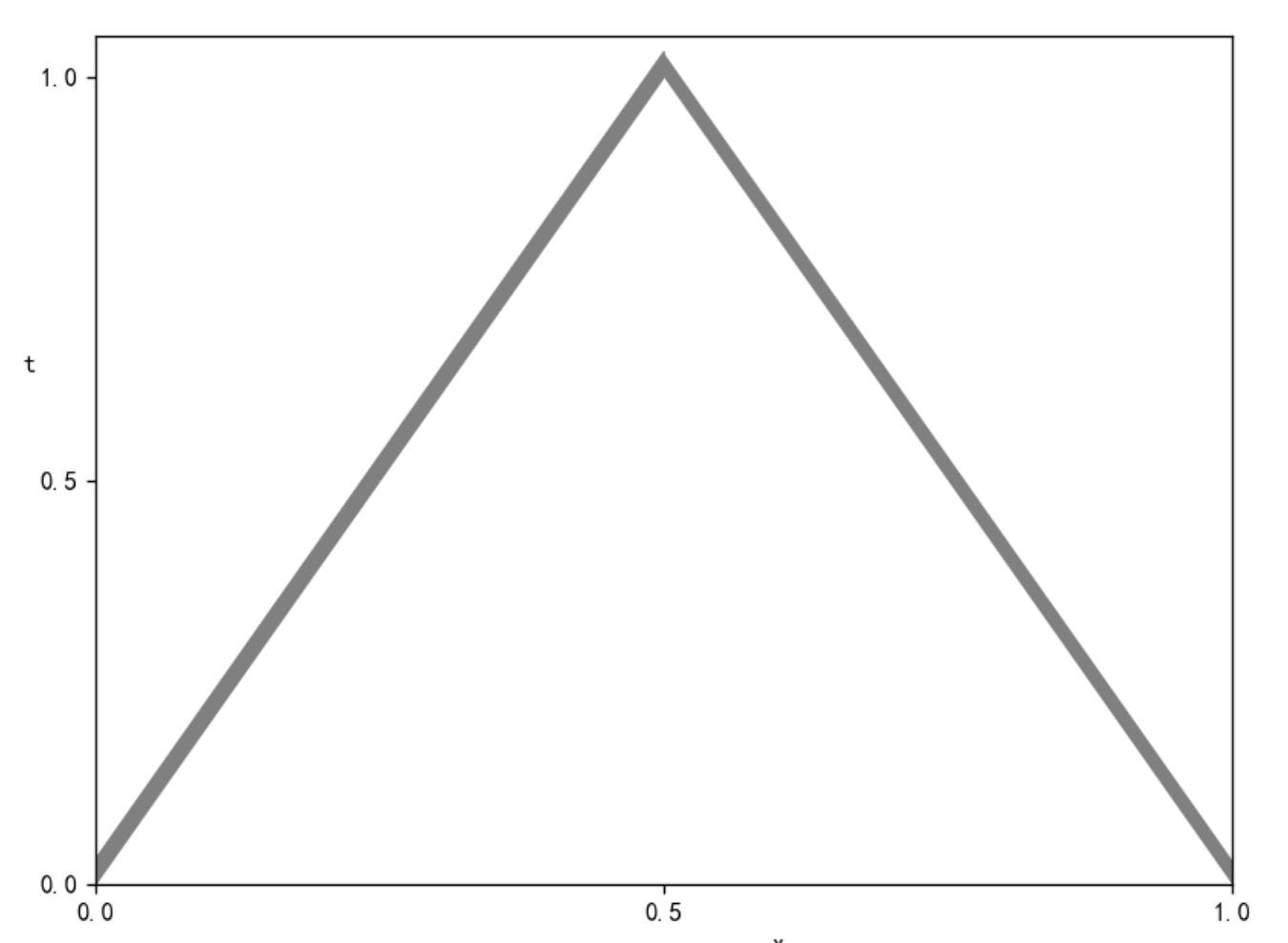
• the hyperbolic component y_h(\cdot;y_0) has the leading term -M(\cdot) A^{-2} y_0, and holds the propagation of singularities along the time direction. More precisely, \forall t_0>0, \forall\, x_0 \in \Omega,

Propagation of singularities
•

y_h(\cdot; y_0) \not\in H^{ \textcolor{purple}{s+4} }_{loc}(t_0,x_0) \Leftrightarrow y_0 \notin H^{ \textcolor{purple}{s} }_{loc}(x_0).

Here, H^r_{loc}(p) means the space of functions each of which is in H^r(\mathcal U_p) for an open neighborhood U_p of the point p.

This allows us to simply call it “wave with the null velocity” (or “static wave”).
Characteristic lines: \{(t, x_0) ~:~ t\geq 0\}, x_0 \in \Omega.

In summary, the model here behaves more like “heat” around the initial time, and more like “wave” at positive time.

 

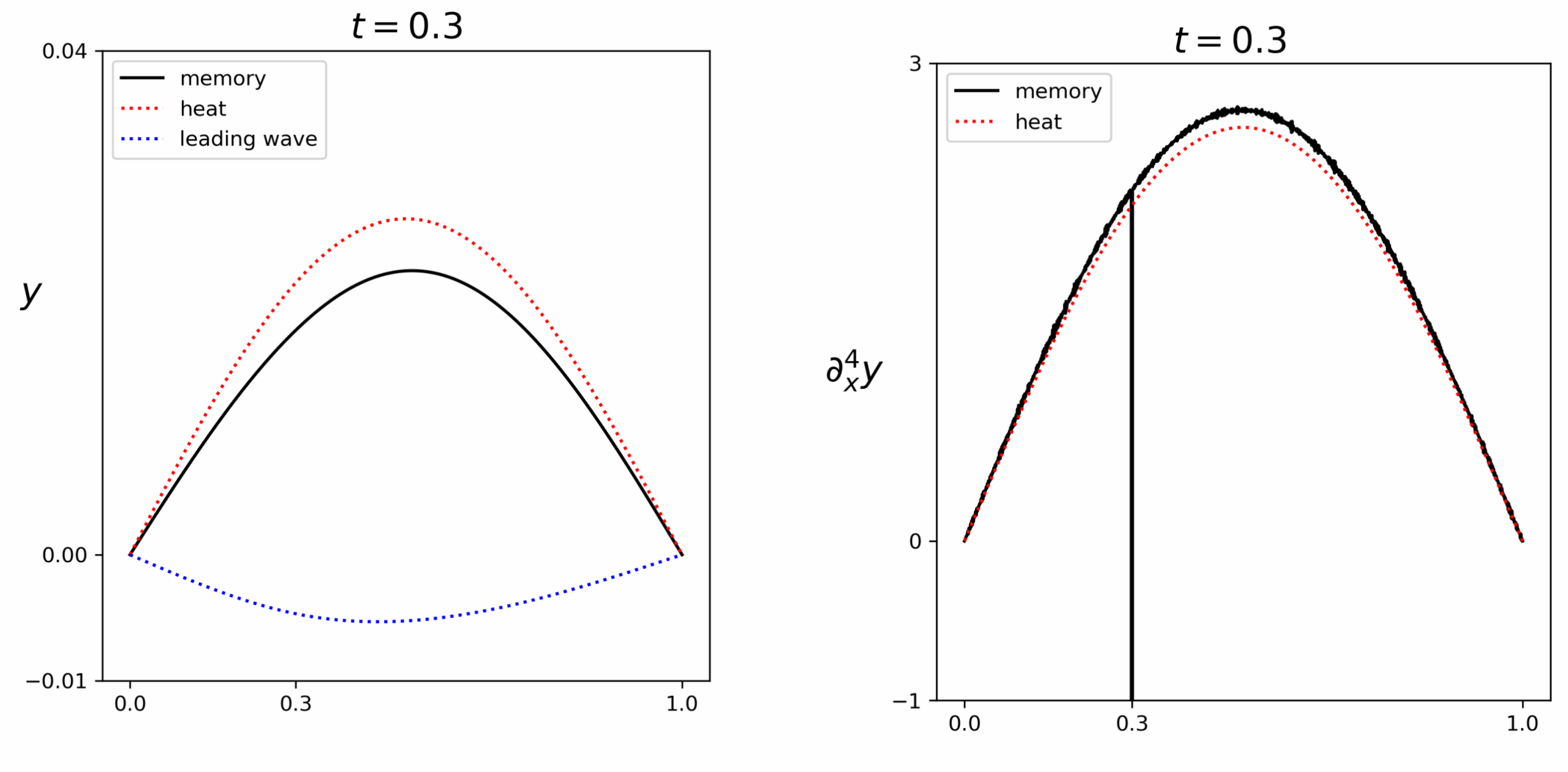
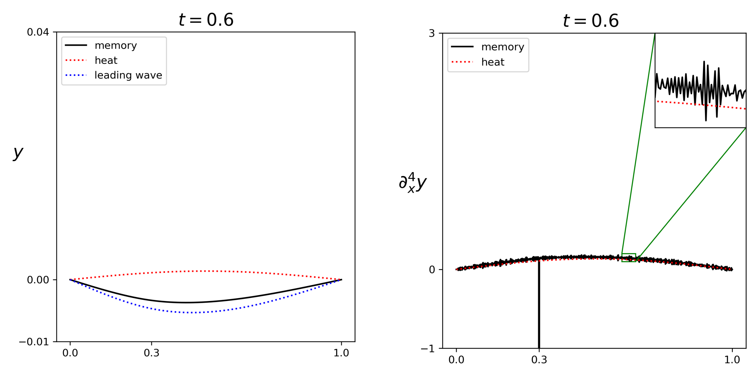
4 Numerical simulations

Let \Omega = (0,1) and y_0 = \delta_{0.3}. The solution and its fourth derivative are drawn in black.

The solution of the pure heat equation with same initial data is drawn in red.

The leading term in the hyperbolic component is drawn in blue.

 

5 Application to observability

(see [2])}
Take a measurable subset Q\subset (0,+\infty) \times \Omega as the observation set.

Moving observation condition

Let T>S\geq 0. The triplet (Q,S,T) is said to satisfy the moving observation condition (MOC for simplicity) if

\mathcal T_{\Omega}(Q,S,T) :=\underset{x\in\Omega}{\text{ess-inf}} \int_S^T \chi_Q(t,x) dt > 0 .

Here, \chi_Q is the characteristic function of Q.

In plain language, the MOC says that each characteristic line goes through the observation set Q\cap\big( (S,T)\times\Omega \big) within a lower-bounded elapsed time. This is comparable to the well-known GCC for observability of wave equations.

When T>S>0, the triplet (Q,S,T) satisfies the MOC
iff
there is a C_1>0 so that

\frac{1}{C_1} \| A^{-2} y_0\|_{ L^2(\Omega) } \leq \int^T_{ S } \big\| \chi_Q(t,\cdot) y(t;y_0) \big\|_{L^2(\Omega)} dt \leq C_1 \| A^{-2} y_0\|_{ L^2(\Omega) } , ~ \forall\,y_0 \in L^2(\Omega) .

When T>S=0 and \alpha>1, the triplet (Q,S,T) satisfies the MOC
iff
there is a C_2>0 so that

\frac{1}{C_2} \| A^{-2} y_0\|_{ L^2(\Omega) } \leq \int^T_{ 0 } \big\| \chi_Q(t,\cdot) y(t;y_0) \big\|_{L^2(\Omega)} \textcolor{red}{t^{\alpha}} dt \leq C_2 \| A^{-2} y_0\|_{ L^2(\Omega) }, ~\forall\,y_0 \in L^2(\Omega)

(the equivalence does not hold any more for \alpha \leq 1).

 

6 Summary

• Memory is a huge perturbation and brings a heavy influence on the nature of the model.
• Memory is “static waves” (with the null velocity). A solution always remembers its past singularities.
• The hyperbolic nature of the memory can help study control problems (such as the controllability and observability problems).

 

7 Open problems

Extensions for general memory kernels:
• Locally integrable memory kernel M\in L^1_{loc}([0,+\infty));
• Space-dependent memory kernel M=M(t,x).

Extensions to more models with memory:
• Memory kernels in the principal part of the model:
• (i) \partial_{t} y - \Delta y - \int _{0}^{t} M(t-s) \Delta y(s)ds=0;
• (ii) \partial_{t} y - \int _{0}^{t} M(t-s) \Delta y(s)ds=0.

• Other equations with memory.

Applications to other problems:
• Other topics such as stabilization, optimal control problems and so on.

 

8 Selected references

[1]\ G. Wang, Y. Zhang, and E. Zuazua. Flow decomposition for heat equations with memory. J. Math. Pures Appl. 158 (2022) 183-215.
[2]\ G. Wang, Y. Zhang, and E. Zuazua. Observability for heat equations with time-dependent analytic memory. Arch. Rational Mech. Anal. 248 (2024): 115.