Transition Layers in Elliptic Equations

Stable transition layers in an unbalanced bistable equation
Consider the following semi-linear problem
$\left\{\begin{array}{ll} u_t=\epsilon^2(k_1^2(x)u_x)_x+k_2^2(x)g(u,x),& (t,x)\in\mathbb{R}^+\times (0,1),\\\\ u_x(t,0)=u_x(t,1)=0,& t\in\mathbb{R}^+, \end{array}\right. (1)$

where $k_1,k_2\in C^1(0,1)$ are positive functions in $[0,1]$ ; $\epsilon$ is a positive parameter and
$g(u,x)=(u-a(x))(b(x)-u)(u-c(x)). (2)$

We assume that the functions $a,b,c$ satisfy
$(g_1)$ $a,b,c\in C^1(0,1)$ ;

(g_2)

a(x)\lt b(x)\lt c(x)

for all

x\in [0,1]

;

(g_3)

there is a sub-interval

[x_1,x_2]\subset [0,1]

such that

b(x)=(a(x)+c(x))/2

for

x\in [x_1,x_2]

and

b(x)> (a(x)+c(x))/2

for all

x\in [0,1]\backslash [x_1,x_2]

The function $g$ is a typical example of the so-called unbalanced bistable function. In this work we prove the existence of a family of stable stationary solutions of (1) that develop internal transition layers as $\epsilon\to 0$ (usually referred to in the literature as stable transition layer). We recall that a stationary solution $u_{\epsilon}$ of (1) is called stable if for every $\eta>0,\;\exists\,\delta>0$ such that for every solution $v_\epsilon$ to (1) satisfying $\|v_{\epsilon}(\cdot\,; 0) - u_\epsilon(\cdot) \|_{L^\infty} \lt \delta$ it holds that $\|v_{\epsilon}(\cdot\,; t) - u_\epsilon(\cdot) \|_{L^\infty}\lt\eta,\; \forall\,t>0.$

Stable nonconstant solutions are often called patterns in the literature, and problems such as those addressed here serve as models for a variety of biological, chemical, and other systems.
For instance, in a process of competition between two species or in the interaction between substances in a chemical reaction or in the heat propagation in heterogeneous materials, the function $k_1$ corresponds to the property of the material where the diffusion phenomenon occurs. In its turn, $k2, a, b, c$ are related to the reaction term on the diffusion process. Roughly speaking, the study of existence of stable solutions can give us the whole dynamics of the parabolic problem and, in this sense, the knowledge of the behavior of solutions when $\varepsilon → 0$ is of great value.
Our main result is the following.

Theorem
Suppose that the function

\gamma(x):=k_1(x)k_2(x)[c(x)-a(x)]^3

assumes at least two isolated local minima $\overline{x}_1,\overline{x}_2$ such that $x_1\lt\overline{x}_1\lt\overline{x}_2\lt x_2$ .

Let $u_0$ be a function defined by
$u_0(x)=a(x)\chi_{(0,\overline{x}_1)}+c(x)\chi_{(\overline{x}_1,\overline{x}_2)}+a(x)\chi_{(\overline{x}_2,1)}. (3)$

Then there exists a sequence $\{u_{\epsilon_j}\}$ ( $\epsilon_j\to 0$ , as $j\to\infty$ ) of stable stationary solutions of (1) such that

u_{\epsilon_j}\to u_0

L^1(0,1)

, as

j\to \infty

A typical solution obtained by this theorem is shown below.

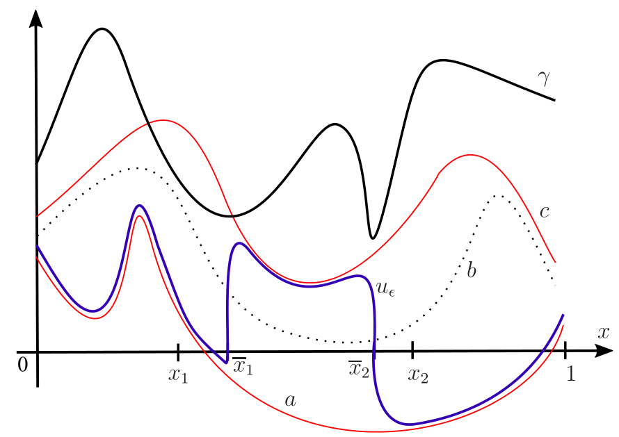
Figure 1.
$u_{\epsilon}$ developing two internal transition layer with interfaces at $\overline{x}_1$ and $\overline{x}_2$ (isolated local minima of $\gamma$ in $[x_1,x_2]$ ).

On the internal transition layer to some inhomogeneous semilinear problems: interface location

When a differential equation contains a small parameter in the spatial derivatives and this parameter goes to zero we, roughly speaking, say that a one-parameter family of solutions develops internal transition layer if it induces a partition in the domain in two regions where, except for a narrow set – the so called interface region of the transition layer – the solutions approach two pre-determined functions (one in each region). Solutions of differential equations developing internal transition layer play an important role in many areas of applied science, for instance: combustion theory, phase transitions, pattern formation, population biology, and chemical reactions.

To know a priori the location of the interface of a family of solutions of a differential equation, in general, is not an easy task and, obviously, this information is very important in the construction of layered solutions.

In this work we contribute to the task of providing the exact location of the interface for some classes of solutions of the following singularly perturbed inhomogeneous problem

\left\{\begin{array}{ll} \epsilon^2(k(x)u'(x))'+f(u,x)=0,\ \ x\in (0,1),\\ u'(0)=u'(1)=0, \end{array}\right. (4)

where $k(\cdot)\in C^1(0,1)$ is positive; $\epsilon>0$ is a positive parameter and $f:\mathbb{R}\times [0,1]\to\mathbb{R}$ is of class $C^1$ .

We assume that
$(f_1)$ $f(\cdot,x)$ has two zeros $b_1(x),b_2(x)$ such that $b_1,b_2\in C^1(0,1)$ and $b_1(x)\lt b_2(x)$ for all $x\in [0,1]$ ;
$(f_2)$ $\partial_1 f(b_1(x),x)\lt0$ and $\partial_1 f(b_2(x),x)\lt0$ for all $x\in [0,1]$ ;
$(f_3)$ if
$F(u,x)=-\displaystyle\int_{b_1(x)}^uf(s,x) ds (5)$

then $F(\cdot,x)\geq 0$ for all $x\in [0,1]$ and $\sqrt{k(\cdot)F(\cdot,\cdot)}$ is Lipschitz continuous.

A typical example of a function $f$ satisfying $(f_1)-(f_3)$ is

f(u,x)=-(u-b_1(x))(u-a(x))(u-b_2(x)), (6)

with $b_1(\cdot), a(\cdot), b_2(\cdot)\in C^1(0,1)$ and $b_1(x)\lt a(x)\lt b_2(x)$ (with $a\geq (b_1+b_2)/2$ ) for all $x\in [0,1]$ . This function is related to inhomogeneous Allen-Cahn problem which has its origin in the theory of phase transitions and is used as a model for many nonlinear reaction-diffusion processes.

The solutions of (4) are the critical points of the energy functional $\tilde{J}_{\epsilon}:H^1(0,1)\to\mathbb{R}$ defined by

\tilde{J}_{\epsilon}(u)=\displaystyle\int_0^1\frac{\epsilon}{2}k(x)|u'|^2+\frac{1}{\epsilon} F(u,x)dx,

where $F$ is defined in (5). However, our main result requires extending this functional to $L^1(0,1)$ ; i.e. we consider $J_{\epsilon}:L^1(0,1)\to\mathbb{R}\cup\{\infty\}$ defined by penalization in $L^1(0,1)$ by

J_{\epsilon}(u)=\left\{\begin{array}{l}\displaystyle\tilde{J}_{\epsilon}(u),\ \ \ u\in H^1(0,1),\\ \infty,\ \ \ u\in L^1(0,1)\backslash H^1(0,1). \end{array}\right. (7)

We are concerned with the role of inhomogeneities of (4) in the location of the internal transition layer of two classes of solutions of (4), namely: $L^1$ -local minimizers of $J_{\epsilon}$ and global minimizers of $\tilde{J}_{\epsilon}$ (which, of course, are also global minimizers of $J_{\epsilon}$ ). We recall that $u_{\epsilon}$ is a $L^1$ -local minimizer of $J_{\epsilon}$ if there exists $\delta>0$ such that $J_{\epsilon}(u_{\epsilon})\leq J_{\epsilon}(u)$ if $||u_{\epsilon}-u||_{L^1(0,1)}\leq\delta$ . Each $L^1$ -local minimizer of $J_{\epsilon}$ is a $H^1$ -minimizer of $\tilde{J}_{\epsilon}$ as well; that is, it is a weak solution of (4). By the theory of regularity, it is a classical solution of (4).

We denote by $\chi_A$ the characteristic function related to set $A$ .

Definition
A family $\{u_{\epsilon}\}$ of solutions of (4) in $C^2(0,1)\cap C^1[0,1]$ is said to develop an internal transition layer, as $\epsilon\to 0$ , with interface at $\overline{x}\in (0,1)$ if
$u_{\epsilon}\stackrel{\epsilon\to 0}{\to}u_0:=b_2\chi_{[0,\overline{x})}+b_1\chi_{[\overline{x},1]} in L^1(0,1).$ (8)

In order to state our main result, we define the following function $\Lambda:(0,1)\to \mathbb{R}$ ,
$\Lambda(x):=\displaystyle\int_{b_1(x)}^{b_2(x)}\sqrt{k(x)F(s,x)}ds (9)$

and the set

\mathcal{Q}=\left\{x\in (0,1); \int_{b_1(x)}^{b_2(x)}f(s,x)ds=0\right\}. (10)

For example, if $f$ is given by (6) then $\mathcal{Q}=\{x\in (0,1); a(x)=(b_1(x)+b_2(x))/2$ }. We say that the points in $\mathcal{Q}$ are that where $f$ satisfies the equal-area condition. It is well known that if $\overline{x}$ is the interface of a family of solutions of (4) developing internal transition layer, then $\overline{x}\in\mathcal{Q}$ . This type of result occurs for several classes of problems and can be a good result of location of interface when, for instance, $\mathcal{Q}$ is discrete. We recall that the equal-area condition also appears in a disguised form by requiring that the potential in the energy functional is of the type double-well.

Our main result is the following.

Theorem
Suppose that a family $\{u_{\epsilon}\}$ of solutions to (4) develop internal transition layer with interface at $\overline{x}\in \mathcal{C}$ , where $\mathcal{C}\subset\mathcal{Q}$ is the connected component of $\mathcal{Q}$ that $\overline{x}$ belongs to. Then,

(i) if $\{u_{\epsilon}\}$ is a family of $L^1$ -local minimizers of $J_{\epsilon}$ ,
$\overline{x} is a local minimum point of \Lambda(x) in \mathcal{C}; (11)$

(ii) if $\{u_{\epsilon}\}$ is a family of global minimizers of $\tilde{J}_{\epsilon}$ ,
$\Lambda(\overline{x})=\min\{\Lambda(x);\ \ x\in\mathcal{C}\}.$

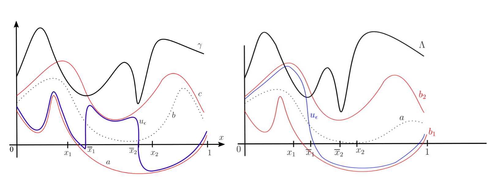
Below we see an illustration of a solution $u_{\epsilon}$ and its internal transition layer, where: $f(u,x)=-(u(x)-b_1(x))(u-a(x))(u-b_2(x))$ , $\mathcal{Q}=[x_1,x_2]$ (i.e. $a(x)=(b_1(x)+b_2(x))/2$ only if $x\in [x_1,x_2]$ ) and $\overline{x}_1,\overline{x}_2$ are local and global minimum points of $\Lambda(\cdot)$ in $[x_1,x_2]$ , respectively. We note that $\{u_{\epsilon}\}$ is a family of $L^1$ -local minimizers of associated functional. If they were global minimizers the interface should be at $\overline{x}_2$ .