
Combined convection and diffusion in a network. A numerical analysis.

The problem: a contaminant in a network of water pipes
Imagine that there is a network of pipes full of water. The water is flowing from some source nodes (say, some water plants) to some destination nodes (say, people’s homes). A contaminant is present in the water (you can imagine it as some coloured ink) and, as time passes, it behaves in two ways:
1. the contaminant diffuses through the water, that is it spreads in the neighbourhood of higher concentration areas;
2. it flows with the stream of water at certain speeds, that have a certain constant value in each pipe (say, the speed depends on the thickness of that particular pipe).
The studied equation quantifies the time evolution of the concentration of the contaminant in the network. Mathematically, it takes the following form:
\begin{cases} \partial_t u_e(t,x) -\delta \partial_{xx} u_e(t,x)+\alpha_e \partial_x u_e(t,x) =0 , & x \in e\in E, t \geq 0; \\ u_{e_1}(t,v) = u_{e_2}(t,v), & v\in V_{\rm int}, e_1,e_2\in E_v,t \geq 0; \\ \sum_{e \in E_v^{\rm in}} \partial_x u(t,v) = \sum_{e\in E_v^{\rm out}} \partial_x u(t,x), & v\in V_{\rm int},t\geq 0; \\ u(0,x)=u_0(x), & x \in \Gamma; \\ u(t,v)=u_v(t), & v \in V_{\partial}, t \geq 0. \end{cases}
Here, V_{\rm int} stands for the set of interior vertices, and the set of boundary vertices is denoted by V_{\partial} (see Figure 1).
The set E_v of the edges adjacent to a vertex v is divided into the set of incoming edges E_v^{\rm in} (e_1 and e_2 in Figure 2) and the set of outgoing edges E_v^{\rm out} (e_3 and e_4 in Figure 1). The function u defined on the graph is the family of all (u_e)_{e\in E}. The diffusivity coefficient \delta is a positive constant.
 Figure 1. An example of tree with input and output boundary vertices (marked with big arrows) and interior vertices (marked with circles).
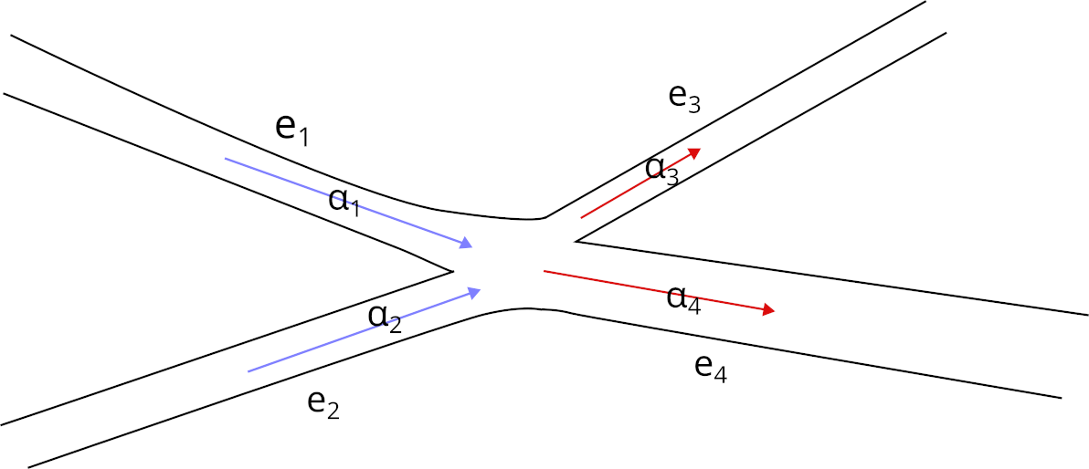 Figure 2. An example of junction in the network. The sum of the incoming speeds (\alpha_1+\alpha_2) equals the sum of the outgoing speeds (\alpha_3+\alpha_4).
Since, on one hand, the liquid cannot accumulate in the junctions and, on the other hand, we want to avoid water shortages, we impose the following conservation condition (see Figure 1) regarding the non-negative speeds \alpha_e corresponding to each edge, at each interior vertex v:
\sum_{e\in E_v^{\rm in}} \alpha_e = \sum_{e\in E_v^{\rm out}} \alpha_e.
Discretising the equation — solving the problem using the computer
In our work, we developed a so-called finite differences numerical scheme for computing the concentration of a contaminant in a network of pipes. We formulated a discrete problem, by considering only a finite number of points on the graph (they are similar to milestones on a highway) and a finite number of time steps. The discrete problem can be solved solely by algebraic computations (which can, in turn, be implemented on a computer) and its result is an approximation of the continuous problem.
During the development of the finite differences scheme, we paid particular attention to the approximation of the continuous problem near the junctions. The biggest challenge was to understand the impact that the combination of incoming and outgoing flows, together with the diffusion behaviour had on the variation in time of the concentration near the junctions. This allowed us to develop suitable computer code to approximate the continuous problem. We proved that this approximation becomes more accurate as the number of chosen milestone points in the pipes increases.
In more mathematical terms, the finite difference scheme is stable provided that the distance between the time steps \tau and the width of the spatial discretisation h (i.e. the distance between the milestones) satisfy the following so-called Courant–Friedrichs–Lewy condition:
\frac{\tau}{h} \max_{e\in E}\alpha_e \lt 1.
The convergence of the finite difference scheme is \mathcal{O}(\tau+h) for regular enough initial and boundary data.
An example output
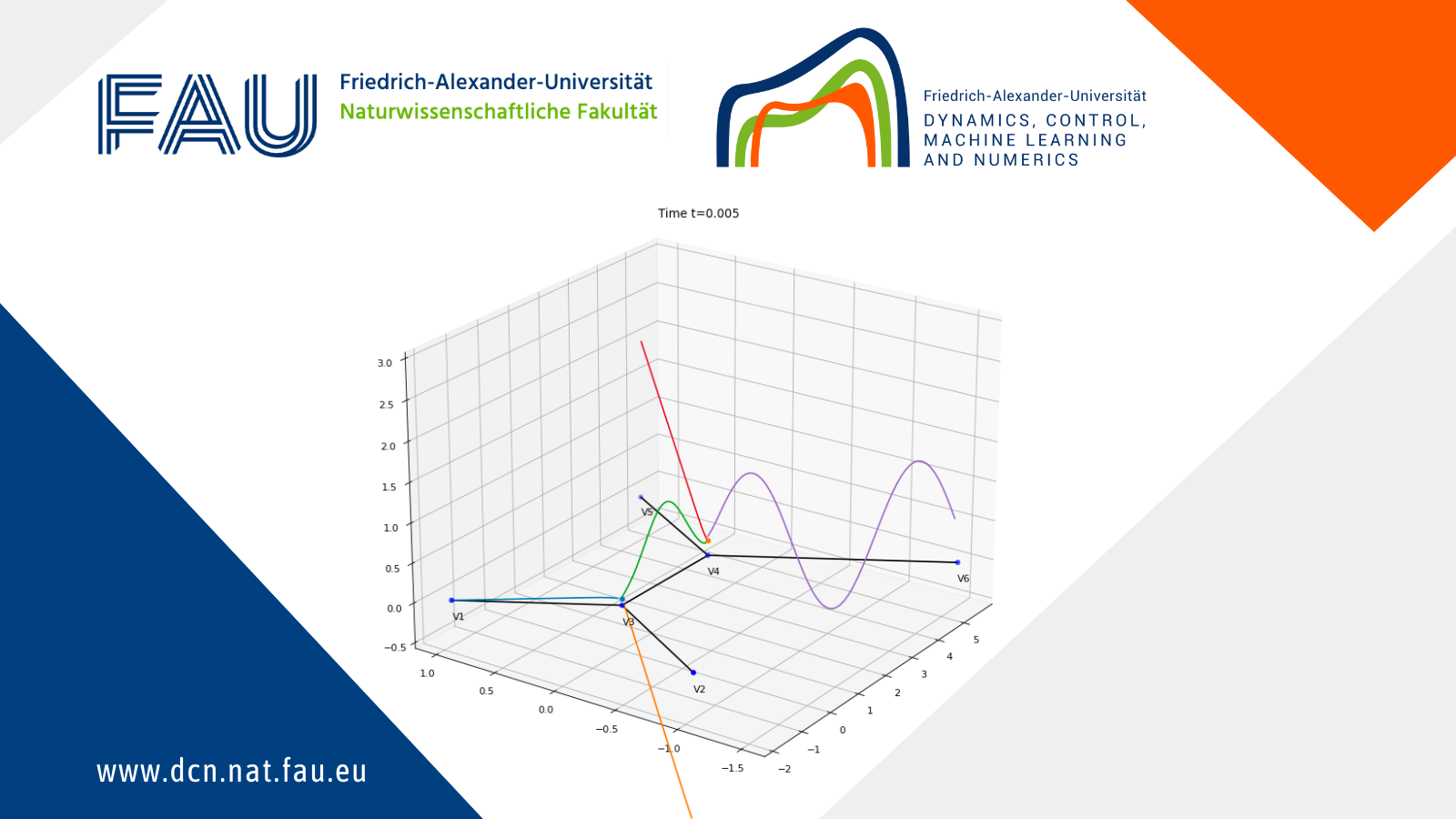
An animation of numerical solution obtained using the algorithm is presented in Figure 3, where the height of the coloured line above a point of the graph on “the floor” represents the concentration of the contaminant in that particular point.
Figure 3. The animation of the solution of the convection-diffusion problem on a network.
GitHub Repository
The code that produced this output can be found in the following GitHub repository from our FAU DCN-AvH GitHub, at: https://github.com/DCN-FAU-AvH/numerical_graphs
Acknowledgements
The author wants to thank COST Action CA18232 – Mathematical models for interacting dynamics on networks for supporting this work.
The author also acknowledges the hospitality of the FAU DCN-AVH Chair for Dynamics, Control, Machine Learning and Numerics in the Department of Mathematics, FAU Erlangen-Nürnberg https://www.fau.de/, where part of this work was carried out.
|| Go to the Math & Research main page


