

HYCO: The hybrid-collapse strategy for time-independent PDEs
 Matthys Jacobus Steynberg
This post explores core ideas on a novel hybrid modelling procedure, within the framework of time-independent partial differential equations, drawn from ongoing research in collaboration with Lorenzo Liverani and Enrique Zuazua.
GitHub Repository
The code to reproduce the experiments can be found at our FAU DCN-AvH GitHub, or directly at:
https://github.com/DCN-FAU-AvH/HYCO-Blog
The structure of the repository is thoroughly explained in the readme document.
1 Introduction
Mathematical models are the tools we use to predict weather, design aircraft, or understand pandemics. Building these models, however, is a delicate art: we must balance what we know about the world with what we can learn from data. There are two main strategies guiding the setup of these models: physics-based and data-driven modeling. Physics-based models are derived from fundamental laws of nature, creating interpretable structures with relatively few parameters. In contrast, data-driven modeling is grounded in modern statistical and machine learning techniques, inferring structure from large datasets without enforcing any physical assumptions.
Physics-based models come with strong theoretical guarantees and are highly interpretable. Data-driven models, meanwhile, are more flexible and easier to use in situations where little is known about the origins of the data. However, this flexibility comes at a cost: they typically require vast amounts of data for training, and their inner workings are seldomly understood.
To address these limitations, hybrid modeling integrates physical insights into data-driven frameworks, leveraging known structure to guide learning. Methods such as Physics-Informed Neural Networks (PINNs), Neural Operators, SINDy, and Latent Dynamics Networks exemplify this approach [1,7,10,9], where the model is trained not only to fit data but also to satisfy assumed physical constraints.
In our work, we propose a new strategy that combines physical and synthetic models. Instead of choosing one of these, we use both models and train them on the data at the same time, while also trying to minimize the distance between their outputs on unseen data. We call this new modeling paradigm “Hybrid Collapse” strategy, or HYCO in short.
In practice, given two models, we work under the assumption that “In medio stat virtus”, meaning that the truth must lie somewhere in between. Hence, rather than choosing one or the other, we optimize the two models to be as close as possible to the data and, crucially, to each other. This mutual alignment is what we call “Collapse”.
The final result of our procedure is thus made of two models, one physical and one synthetic. Both are optimized on the data, but each one is biased by the other to agree also outside of distribution. This is also why we talk about a “strategy” and not of a HYCO “model”. This approach offers two main advantages:
(1) For online evaluation we now have two choices. We can either use the mathematically precise, but slower physical model, or the lighter synthetic model. Our training procedure ensures that both the physical and the synthetic output will be similar.
(2) The interaction between the two models might improve situations in which data is scarce, noisy or localized. Indeed, each model acts as a regularization to the other.
2 Experiment 1: The Poisson Equation
2.1 Experimental setup
We will introduce this approach by means of an example. To this end, we consider as ground-truth model the 2D Poisson equation with homogeneous Dirichlet boundary conditions [3].
The governing equation is
\begin{dcases} - \Delta u = f(x, y), & \text{for } (x, y) \in \Omega, \\ \boldsymbol{u}(x, y) = 0, & \text{for } (x, y) \in \partial\Omega, \end{dcases} \hspace{0.5cm} (2.1)
where \Omega = [-\pi, \pi]^2.
We define the reference solution as
\boldsymbol{u}(x,y) = \sin(x)\sin(y), \hspace{0.5cm} (2.2)
by choosing the forcing term
f(x,y) = A\sin(k_x x)\sin(k_y y), \hspace{0.5cm} (2.3)
with A = 2, k_x = 1, and k_y = 1.
The experiment is then set up as follows.
• The physical model is taken to be the Poisson equation (2.1), where the parameters of the forcing term,
\Lambda = \{A, k_x, k_y\},
are unknown.
In practice, we will use a Finite Element approximation of this model, computed on a 20\times20 equispaced grid.
• The synthetic model to be a fully connected neural network, with 256 neurons, 2 layers, and the ReLU activation function. Accordingly, the set of parameters \Theta consists in the neural network weights and biases.
The objective of this experiment is thus to optimize the parameters \Lambda and \Theta to match the sensors’ observations.
2.2 The Collapse Strategy
Before describing the algorithm in detail, we first formalize the notion of “collapse”. Consider two types of sensor positions on the domain, namely
• \{\mathbf{x}_i\}, the positions of real sensors, where data from the reference solution is known.
• \{\mathbf{x}_G\}, the positions of “ghost” sensors, where data from the reference solution is not known.
The necessity of these “ghost” sensors will become clear once we introduce the interaction loss term. However, firstly we begin by looking at the general procedure to train the parameters \Theta of a neural network using the known data. This consists of minimizing the loss function
L_{syn}(\Theta) = \frac{1}{M}\sum_{i = 1}^M\|\boldsymbol{u}_\Theta(x_i) - \boldsymbol{u}^D(x_i)\|^2,
where \boldsymbol{u}_D is the reference solution, and \boldsymbol{u}_\Theta is the solution of the synthetic model.
Similarly, one can train the parameters \Lambda of the physical model by solving the minimization problem
\min_{\Lambda} L_{phy}(\Lambda) := \frac{1}{M}\sum_{i = 1}^M\|\boldsymbol{u}_{\Lambda}(x_i) - \boldsymbol{u}^D(x_i)\|^2
\text{subject to} \quad \boldsymbol{u}_{\Lambda}(x) \text{ solve } (2.1).
At this point, we observe that both models are defined at every point in \Omega. Therefore, we can compare the value of \boldsymbol{u}_\Lambda not only to the data u^D(x_i), but also to the approximation provided by the synthetic model.
We thus introduce the interaction loss
L_{int} = \frac{1}{H}\sum_{h=1}^H \|\boldsymbol{u}_\Theta(x^G) - \boldsymbol{u}_\Lambda(x^G) \|^2,
which compares the models on these so-called “ghost” sensor positions.
In conclusion, we can finally propose the HYCO strategy as
\begin{aligned} &\min_{\Theta, \Lambda} &&L := \alpha L_{syn}(\Theta) +\beta L_{phy}(\Lambda) + L_{int}(\Theta, \Lambda) \\ &\text{subject to} \quad && \boldsymbol{u}_\Lambda \text{ solves } (2.1). \end{aligned} \hspace{0.5cm} (2.4)
Here \alpha,\beta are two weights that can be tuned to give more importance to the synthetic model, the physical model, or the interaction between the two.
2.3 The Training Algorithm
Now we are able to describe the training algorithm in detail.
Step 1: Collecting the Data.
We randomly fix the position of 25 sensors and evaluate the analytical solution at these positions. The final result is a set of 25 data points \mathcal{D} = \{\boldsymbol{u}^D(x_i,y_i)\}_{i=1}^{25}.
Step 2: Initialization.
The unknown parameters are initialized randomly. In particular, the physical parameters used for our experiment have the values
A = 0.948 , k_x = 0.979, k_y = 0.332
The parameters \Theta of the neural network are initialized following a normal distribution with variance scaling [5].
Step 3: Training the models.
This step is the core of the algorithm. The models are trained using stochastic gradient descent. However, we alternate the gradient descent step sequentially between the physical model and the synthetic one. More specifically, at each epoch we perform the following steps:
(1) Place 200 ghost sensors (H = 200) randomly within the domain. These will be used to compute the interaction loss.
(2) Perform a gradient descent step to minimize the sum \mathsf{L}_{syn} + \mathsf{L}_{int} over \Theta, while the parameters of the synthetic model are kept fixed.
(3) Perform a gradient descent step to minimize the sum \mathsf{L}_{phy} + \mathsf{L}_{int} over \Lambda, while the parameters of the physical model are kept fixed.
We train for a total of 3000 epochs.
For clarity, the training of the models is shown in animation 2.1.
Figure 2.1. A depiction of the training algorithm.
3 Experiment 2: The Helmholtz Equation
After introducing the HYCO strategy with the simple Poisson example, we now consider a more challenging experiment based on the Helmholtz equation. This experiment is divided into two parts: first, we validate HYCO’s ability to learn PDEs from sensor data scattered throughout the domain; second, we compare HYCO to two classical techniques, the inverse problem and the PINN approach (see Appendix 1 for details), where data is localized to a certain region of the domain.
After training, we evaluate the approximated solution produced by the synthetic and physical models. Note that, for what concerns the latter, we can use the trained parameters to evaluate the solution on a finer grid to produce a high-precision prediction. The predicted solution of the synthetic and physical models after training is shown in figure 2.2.
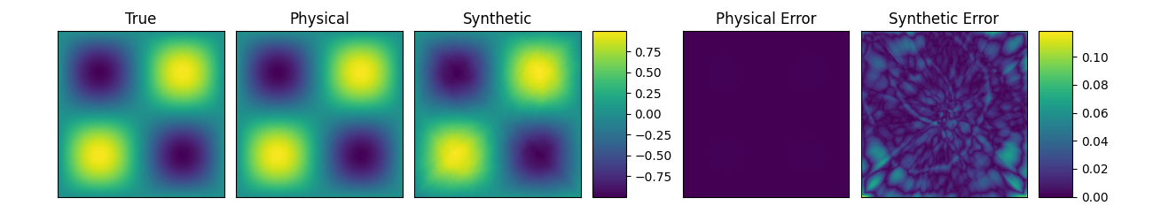
Figure 2.2. Ground-truth solution and approximated solution of the Poisson equation (2.1), obtained through the HYCO strategy.
We consider the 2D heterogeneous Helmholtz equation with null Dirichlet boundary conditions as the ground-truth model [4]. The inverse problem for this time-independent partial differential equation (PDE) frequently arises in the context of medical and seismic imaging, in particular, in the method of full waveform inversion [8].
The governing equation is
\begin{dcases} - \nabla \cdot (\kappa(x, y) \nabla \boldsymbol{u}) + \eta(x, y)^2 \boldsymbol{u} = f(x, y), & \text{for } (x, y) \in \Omega, \\ \boldsymbol{u}(x, y) = 0, & \text{for } (x, y) \in \partial\Omega, \end{dcases} \hspace{0.5cm} (3.1)
where \Omega = [-\pi, \pi]^2.
We set the reference solution to be equal to
\boldsymbol{u}(x,y) = \sin(x)\sin(y). \hspace{0.5cm} (3.2)
The coefficients \kappa(x, y) and \eta(x, y), respectively known as diffusion term and wave number, are modeled as
\kappa(x, y) = \varphi(x,y;\alpha_1,c_1) + 1, \quad \eta(x, y) = \varphi(x,y;\alpha_2,c_2) + 1,
where \varphi(\cdot,\cdot;\alpha,c) is the gaussian function of amplitude \alpha and center c, namely,
\varphi(x,y;\alpha,c) = \alpha e^{-(x-c_x)^2 - (y - c_y)^2}.
The true parameters are chosen to be
\alpha_1 = 4, \quad \alpha_2 = 1, \quad c_1 = (-1, -1), \quad c_2 = (2, 1).
Given this choice and that the reference solution is (3.2), the forcing term is set accordingly. After streightforward, but tedius calculations, we find
\begin{aligned} f(x,y) &= 2(x+1)\,\varphi(x,y;4,(-1,-1))\cos(x) \sin (y) \\ &+ 2(y+1)\,\varphi(x,y;4,(-1,-1))\sin (x) \cos (y) \\ &\left[(\phi(x,y;1,(2,1)) + 1)^2 + 2(\phi(x,y;4, (-1,-1)) + 1)\right]\sin(x)\sin(y). \end{aligned} \hspace{0.5cm} (3.3)
Having settled the ground-truth, we are in position to set up the experiment.
With the same notation of the Poisson experiment, we take:
• The physical model to be the Helmholtz equation (3.1). We assume to know the forcing term (3.3) as well as the gaussian structure of \kappa, \eta, but not the parameters
\Lambda := \{\alpha_1, \alpha_2, c_1, c_2\}.
In practice, we will use a Finite Element approximation of this model, computed on a 20\times20 equispaced grid.
• The synthetic model to be a fully connected neural network, with 256 neurons, 2 layers, and the ReLU activation function. Accordingly, the set of parameters \Theta consists in the neural network weights and biases.
The objective of this experiment is thus to optimize the parameters \Lambda and \Theta to match the sensors’ observations.
We train the models using the same algorithm described in the Poisson experiment. After training, we evaluate the approximated solution produced by the synthetic and physical models. The predicted solution of the synthetic and physical models after training is shown in figure 3.1.

Figure 3.1. Ground-truth solution and approximated solution of the Helmholtz equation (3.1), obtained through the HYCO strategy.
Comparison.
We perform two experiments. In the first one, we take 25 equally spaced sensors in [-3,3]\times[-3,3] (so that all data points are in the interior of \Omega). In this setting, we expect the performance of HYCO to be similar to a simple parameter fitting and to PINNs. We summarize the result in Animation 3.2, where we have evolution of the recovered coefficients \kappa,\eta in the first two lines, as well as the behavior of the error computed as the L^2 norm of the difference between the predicted solution and the real solution while training. In particular, for the classical inverse problem and the PINN we have (in blue and orange)
\mathsf{e}_{inv}:= \|\boldsymbol{u}(x,y) - \boldsymbol{u}_{inv}(x,y)\|_{L^2}^2, \quad\mathsf{e}_{PINN}:= \|\boldsymbol{u}(x,y) - \boldsymbol{u}_{PINN}(x,y)\|_{L^2}^2,
whereas for the HYCO strategy we plot (in green and red)
\mathsf{e}_{phy}:= \|\boldsymbol{u}(x,y) - \boldsymbol{u}_{phy}(x,y)\|_{L^2}^2, \quad \mathsf{e}_{syn}:= \|\boldsymbol{u}(x,y) - \boldsymbol{u}_{syn}(x,y)\|_{L^2}^2.
As expected, with several data points spread throughout the domain, the inverse problem works very well. The PINN seems to struggle, although this might be due to the fact that more training epochs or hyperparameter tuning is required. Both models trained following the HYCO strategy also perform well, though it seems like more epochs would be needed to converge and attain a similar error to the inverse problem. This behaviour is expected: in settings where a direct parameter estimation would perform well, the addition of a synthetic model acts more as a perturbation, at least until a good agreement with the physical model is reached.
In the second experiment, instead, we test the abilities of the models to recover the correct coefficients from localized data. Specifically, now we employ 25 sensors, placed randomly in the square [0,3]\times[0,3], meaning that we have no knowledge of the solution outside of this region.
The results are shown in Animation 3.3. As we can see, every strategy is able to learn the parameter \eta. This is somewhat expected, since \eta is affecting a region of the solution in which we have a lot of data. On the other hand, \kappa affects the region without data. Nevertheless, using the HYCO strategy we are able to recover the correct center of the gaussian for \kappa, whereas both PINN and the classical inverse problem cannot. Accordingly, HYCO is able to achieve the better precision. This is also reflected by the error: the models trained with the HYCO strategy are the only ones capable of decreasing the error, which increases for the other two models instead.
Figure 3.2.
Top: The obtained values for \kappa (top row) and \eta (bottom row) in the Helmholtz equation (3.1): classical inverse problem (first column), PINNs (second column), HYCO (third column). The fourth column is the plot of the ground-truth parameter. In red, the positions of the sensors.
Bottom: Behavior of the L^2 error for the three models. For readability, we plot the moving average of the error over 100 epochs.}
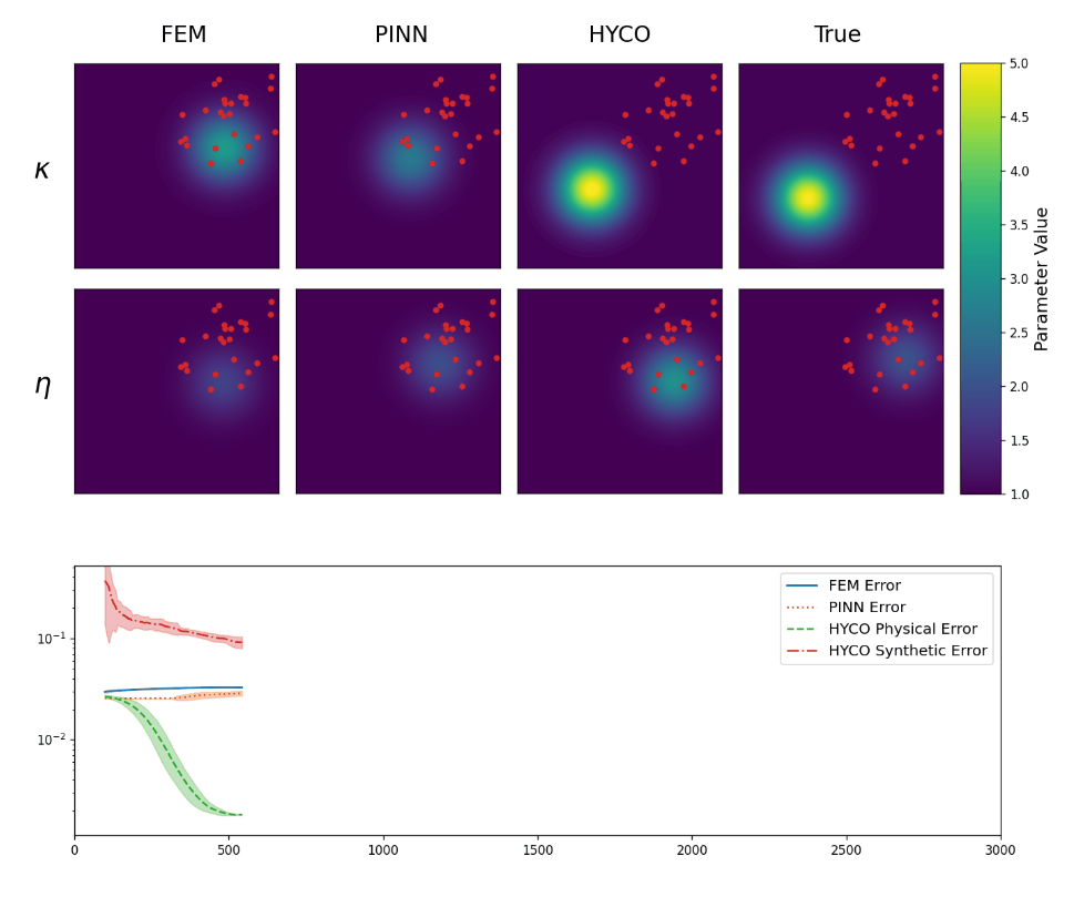
Figure 3.3. Comparison of the recovered coefficients and of the errors for the Helmholtz equation (3.1), in the case of localized data.
Conclusions
In this work, we introduced HYCO, a hybrid modeling strategy that integrates physical and data-driven models by optimizing them simultaneously while enforcing consistency between their predictions. This approach differs from classical inverse problems, which rely solely on parameter estimation within a fixed physical framework, and from PINNs, which incorporate physical constraints into a neural network loss function. Instead, HYCO establishes a two-way interaction: both models influence and regularize each other. This mutual interaction enhances generalization, especially when data is scarce, noisy, or highly localized.
Our numerical experiments demonstrate that HYCO achieves more accurate parameter recovery and superior predictive performance compared to traditional approaches. In particular, HYCO proves highly effective when observations are restricted to specific regions, leveraging the interplay between models to reconstruct missing information.
References
[1] S. L. Brunton, J. L. Proctor, J.N. Kutz (2016) Discovering governing equations from data by sparse identification of nonlinear dynamical systems. Proceedings of the National Academy of Sciences, Vol. 113, No. 15, pp. 3932–3937[2] S. Cuomo, V. Di Cola, F. Giampaolo, G. Rozza, R. M., F. Piccialli (2022) Scientific machine learning through physics–informed neural networks: Where we are and what’s next. Journal of Scientific Computing
[3] L. C. Evans (2010) Partial Differential Equations, Graduate Studies in Mathematics. American Mathematical Society, 2nd edition, Vol. 19, See p. 19.
[4] I. Graham, O. Pembery, E. Spence (2019) The helmholtz equation in heterogeneous media: A priori bounds, well-posedness, and resonances. Journal of Differential Equations, Vol. 266, No. 6, pp. 2869–2923
[5] B. Hanin, D. Rolnick (2018) How to start training: The effect of initialization and architecture. In S. Bengio, H. Wallach, H. Larochelle, K. Grauman, N. Cesa-Bianchi, and R. Garnett, editors, Advances in Neural Information Processing Systems, Vol. 31. Curran Associates, Inc.
[6] E. Kharazmi, Z. Zhang, G.E. Karniadakis (2019) Variational physics-informed neural networks for solving partial differential equations
[7] N. Kovachki, Z. Li, B. Liu, K. Azizzadenesheli, K. Bhattacharya, A. Stuart, and A. Anandkumar (2024) Neural operator: learning maps between function spaces with applications to pdes. J. Mach. Learn. Res., Vol. 24, No. 1
[8] F. Lucka, M. Perez-Liva, B.E. Treeby, B.T. Cox (2021) High resolution 3d ultrasonic breast imaging by timedomain full waveform inversion. Inverse Problems, Vol. 38, No. 2, pp. 025008
[9] M. Raissi, P. Perdikaris, G. Karniadakis (2019) Physics-informed neural networks: A deep learning framework for solving forward and inverse problems involving nonlinear partial differential equations. Journal of Computational Physics, Vol. 378, pp. 686–707
[10] F. Regazzoni, S. Pagani, M. Salvador, L. Dede, A. Quarteroni (2024) Learning the intrinsic dynamics of spatiotemporal processes through latent dynamics networks. Nature Communications, Vol. 15, No. 1, pp. 1834
Appendix 1: The models used for comparison.
1. The classical inverse problem.
Inverse problems are one of the oldest approaches in mathematical modeling. The idea is to optimize the coefficients of a physically-derived PDE to match the observations. In our context, this is exactly equivalent to the minimization of only the loss \mathsf{L}_{phy}. This can be done by gradient descent.
Our first aim is to understand whether the introduction of the synthetic model and of the interaction term in the loss provides a better provide a better approximation of the unknown parameters, with respect to a simple inverse problem.
2. The PINN approach.
Physics-Informed neural networks are a very popular machine learning architecture which aims to learn the solution to a PDE by requiring
that the neural network not only matches the data, but is also “close” to the solution of a certain PDE (ideally the ground-truth underlying the data).
To understand the idea behind PINNs, suppose data is generated by the static problem /textcolor{red}{(??)}. A PINN is a function \boldsymbol{v}_\Theta(x), depending on a set of parameters \Theta, which are tuned to minimize the following loss
\mathsf{L}_{PINN}(\Theta,\Lambda) = \frac{1}{M}\sum_{i=1}^M \|\boldsymbol{v}_\Theta(x_i) - \boldsymbol{u}^D(x_i)\|^2 + \|\mathscr{F}(\kappa)\boldsymbol{v}_\Theta - f\|_{L^2(\Omega)} + \|\mathscr{G}(\lambda)\boldsymbol{v}_\Theta\|_{L^2(\partial\Omega)},
where \Lambda is the set of unknown physical parameters.
On an intuitive level, a PINN penalizes the distance of the neural network from a solution to the PDE ansatz.
PINNs have demonstrated good performances in a plethora of applications. Nevertheless, it has become clear very soon that the approach has limits. For once, the neural network has to be smooth enough if the goal is to optimize the loss above, since \mathscr{F}, \mathscr{G} are differential operators. This problem was solved with the introduction of Variational PINNs (VPINNs) [6]. Still, PINNs remain quite difficult to train, often requiring a fine hyperparameter tuning to obtain good results [2].
|| Go to the Math & Research main page


