
pyGasControls Framework
By Martin Gugat, Enrique Zuazua, Aleksey Sikstel
In order to optimize the operation of gas transportation networks, as a first step a powerful simulation software is mandatory. The flow model from continuum mechanics leads to a nonlinear hyperbolic system of balance laws for each pipe. For the dynamics of the system, the friction term that models the pressure loss in the flow along the pipe is essential. In order to be able to cope with large network graphs, a 1-dimensional moddel is used for each pipe. This allows to arrive at a coupled model on the network by suitable coupling conditions at each node of the graph. It is well-known that in nonlinear hyperbolic systems, the regularity of the solution can degenerate after finite time. Even when the initial state is smooth, shocks can evolve after finite time. The software pyGasControl is able to simulate the pde solutions accurately even if shocks occur.
The pyGasControls framework allows to simulate and compute optimal controls for networks of one-dimensional hyperbolic conservation laws. The software toolbox is implemented in Python allowing it to use a large variety of libraries and interact with existing solvers for hyperbolic conservation laws such as claw1darena, Petsc, openfoam and any other solver that is able to interact with Python. Furthermore, it features arbitrary network graphs that may be set up either directly or using the XML-format defined in the GasLib library. pyGasControls provides an interface for the node conditions of the network allowing to set arbitrary coupling conditions that again might come from an external software package. Finally, the code is easily parallelisable for large scale computations. The source code as well as the documentation of the software is available!
Feedback laws for the p-System on a diamond-shaped network
In particular, we aim for optimal controls of gas networks where the dynamics inside a pipe (i.e. an edge of the network with the index (_e) is modeled by the one-dimensional isothermal Euler equations
\begin{aligned}
&(\rho_e)_t + (q_e)_x = 0\\
&(q_e)_t + \left( \frac{(q_e)^2}{\rho_e} + c \rho_e \right)_x = -\frac12(\theta_e + w_e(x))\frac{q_e|q_e|}{\rho_e}
\end{aligned}
with the following notation:
- (\rho_e) – density in pipe (_e)
- (q = \rho v) – momentum in pipe (_e) where (v_e) – velocity
- (c) – speed of sound
- (\theta) – friction parameter in pipe (_e)
- (w_e(x)) – perturbations of the friction parameter in pipe (_e)
The system (1) is given in conservative form \mathbf{u}_t + (\mathbf{f}(\mathbf{u}))_x = \mathbf{S} with conserved quantities \mathbf{u}:= (\rho_e, q_e)^T, flux function \mathbf{f} and source term \mathbf{S}.
A smooth function R \,\colon\, \Omega \to \mathbb{R} is called an i-Riemann Invariant if
\nabla R(u) \cdot r_i(u) = 0
where r_i is the eigenvector corresponding to the i – th eigenvalue of the Jacobian of the flux \mathbf{f} sorted in ascending order.
In absence of a source term the Riemann invariants are constant along characteristics and across rarefaction waves. The Riemann invariants of the isothermal Euler equations read
R_{\pm}(p, q) = \ln(p) \pm \sqrt{c}\frac{q}{p}We consider a network consisting of E edges. The dynamics of the isothermal Euler equations is computed by the third-order CWENO scheme implemented in claw1darena [1].
For the nodes of the gas network we consider junctions and boundary conditions for the leafs. Given the directional vector of each pipe \nu_e outgoing of a node, the junction coupling conditions are given by
- Mass conservation \sum_{e=1}^E \|\nu_e\| q_e(t,0+) = 0
- Dynamic pressure continuity |\nu_e| P((\rho_e, q_e)(t, 0+)) = P^* (\forall e\in {1,\ldots,E})
- Non-decreasing entropy \sum_{e=1}^E |\nu_e |F((\rho_e, q_e)(t, 0+)) \leq 0
The states that fulfill the conditions (M), (P) and (E) are given via Lax-curves of the half-Riemann problems for each pipe adjacent to a junction node, see [2].
The boundary leaves can be set arbitrary, as a function of the solution of the adjacent pipe. For instance, the boundary leaves can represent feedback boundary controls that stabilize the flow in the system and allow to investigate the decay of Lyapunov-functions of the flow in the network. One interesting example of a feedback law are the Riemann feedback laws, investigated by Coron. The idea is to set the ingoing Riemann invariant to a fraction of the outgoing Riemann invariant.
Simulation of diamond-shaped network
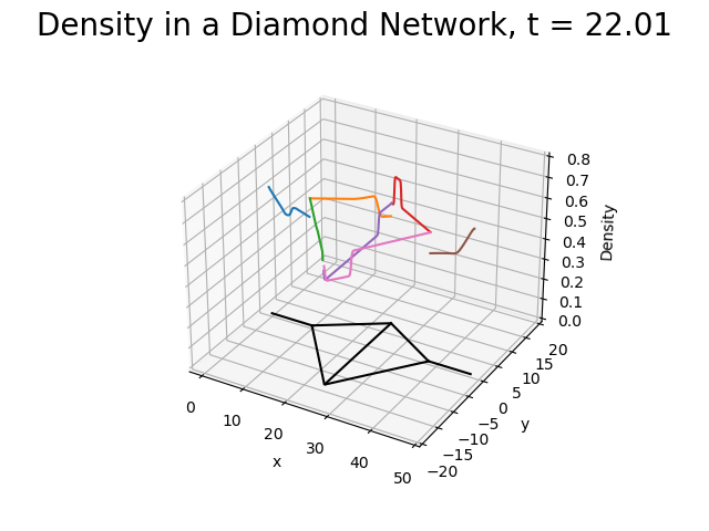
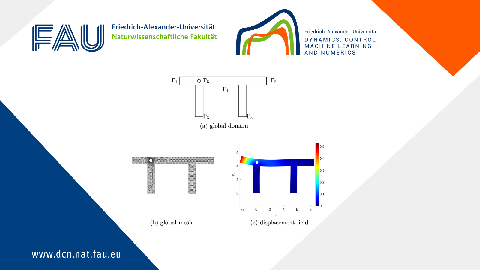
The diameter of the pipes is chosen as 1m constantly across the network and the geometry is presented in Figure 1.
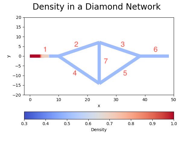
Figure 1.The density of the diamond-shaped network after one timestep.
The initial conditions are chosen as following
\begin{matrix}
\rho_1 \\ q_1
\end{matrix}
=
\begin{cases}
(1, 0)^T & \text{if } x < 5m\\
(0.5, 0)^T & \text{otherwise}
\end{cases},\quad
\begin{matrix}
\rho_e \\ q_e
\end{matrix}
= (0.5, 0)^T, \text{where } e \in\{2,\ldots,7\}.
The boundary leaves of the edges 1 and 6 are set to outflow boundary conditions via Riemann invariants, i.e.
R^+(\rho^{BC}_e, q^{BC}_e)^T = R^+(\rho^{0}_e, q^{0}_e) where the superscript (^+) denotes the Riemann invariant entering the domain and the conservative variables superscript ^0 are located adjacent to the boundary.The dynamics on each edge is obtained numerically by a 3-stage RK CWENO3 method [1], i.e. order (p=3), with (\Delta x = 0.1m) and CFL-number (0.9) until the final time (T=100).
The node dynamics are obtained according to [2] by solving the equations (M) and (P) by a nonlinear Broyden-solver from the library SciPy in every timestep. (Note that inequality (E) is fulfilled at least locally).

Figure 2.This is the placeholder for the video.
WIP: feedback laws comparisons and corresponding figures
Simulation of an example from the GasLib library
WIP: geometry image gaslib11, video shock traveling through gaslib11
Outlook
Control functions might be set in the boundary leaves and the optimal control of the system is then calculated employing a backward solver where the adjoint is chosen as presented in [3]. As the next step, one could consider controls of compressor nodes with constraints on the boundary leaves that represent customers of the gas network owner.
Download the pyGasControl library
[HINT] In order to run the software on your computer, you may have to install additional standard software packages (like cmake and a c++ compiler) and additional libraries (for example lapack, PETSc).
References
[1] Semplice, M., & Visconti, G. (2020). Claw1darena.[2] Colombo, R. M., & Garavello, M. (2008). On the Cauchy problem for the P-system at a junction. SIAM J. Math. Anal., 39(5), 1456–1471. http://dx.doi.org/10.1137/060665841
[3] Herty, M., & Sachers, V. (2007). Adjoint calculus for optimization of gas networks. Networks and Heterogeneous Media, 2(), 733–750. http://dx.doi.org/10.3934/nhm.2007.2.733
|| Go to the Math & Research main page


