
A Turnpike Result for Optimal Boundary Control Problems
with the Transport Equation under Uncertainty
 Noboru Sakamoto
 Michael Schuster
1 The Deterministic Optimal Control Croblem
We consider a deterministic optimal boundary control problem governed by a linear transport equation with source term and the corresponding static optimal problem. We state an integral turnpike result for the optimal controls in the sense that the dynamic optimal control converges to the static optimal control if the time horizon tends to infinity.
For (t,x) \in [0,T] \times [0,L], for initial data r_{ini}(x) \in L^2(0,L), for boundary control u(t) \in L^2(0,L) and for sound speed c>0 consider the linear transport equation with initial and boundary control
\left\{ \quad \begin{aligned} &r_t(t,x) + c r_x(t,x) = m r(t,x), \\ &r(0,x) = r_{ini}(x), \\ &r(t,0) = u(t), \end{aligned} \right. (1)
where r_t(t,x) is the time derivative of r and r_x(t,x) is the space derivative of r. If the sound speed c would be negative the information would be transported the other way around and we would have to assume boundary control at x=L. The constant m is a real number. Note that the linear transport equation (1) is exactly controllable if T \geq L/c. Let convex and differentiable functions
f, g : \mathbb{R} \rightarrow \mathbb{R}_{\geq 0},
be given. For u \in L^2((0,L) and w: L^2(0,T) \rightarrow L^2(0,T) we define the function
\begin{aligned} &J_T : L^2(0,T) \rightarrow \mathbb{R}, &J_T(u) = \int_0^T f\Big(u(t)\Big) + g\Big(w\big(u(t)\big)\Big)\ dt. \end{aligned} (2)
Note that J_T is convex due to the convexity of f and g. For w(u) = r(t,L) we consider the dynamic optimal boundary control problem
\left\{ \quad \begin{aligned} \min_{u \in L^2(0,T)} \quad &J_T(u) = \int_0^T f\big(u(t)\big) + g\big(r(t,L)\big)\ dt \\ \text{s.t.} \quad &r_t(t,x) + c r_x(t,x) = m\ r(t,x), \\ &r(0,x) = r_{ini}(x), \\ &r(t,0) = u(t). \end{aligned} \right. (3)
We consider the static optimal control problem corresponding to (3) that is given by
\left\{ \quad \begin{aligned} \min_{u \in \mathbb{R}} \quad & f(u) + g(r(L)), \\ & c r_x(x) = m r(x), \\ & r(0) = u. \end{aligned} \right. (4)
Before we state the first Turnpike result we make the following assumptions:
• [(A1)] Let the functions f and g satisfy the property
\big( f'(x_1) - f'(x_2) \big) \big( x_1 - x_2 \big) + \big( g'(y_1) - g'(y_2) \big) \big( y_1 - y_2 \big)\ \geq\ \varepsilon\ \Vert x_1 - x_2 \Vert_2^2, (5)
with constant \varepsilon > 0.
• [(A2)] Let the derivative of g be Lipschitz continuous with Lipschitz constant L_k, i.e.,
\Vert g'(y_1) - g'(y_2) \Vert_2\ \leq\ L_k\ \Vert y_1 - y_2 \Vert_2. (6)
The assumption (A1) is essential for the existence of optimal controls in terms of the Direct Method of Calculus of Variations, it holds e.g. if f is strongly convex. Assumption (A2) is necessary for obtaining the time independent turnpike constant.
Theorem 1
Let the assumptions (A1) and (A2) be satisfied. Then there exist optimal controls u^\delta(t) of the dynamic optimal boundary control problem (3) and u^\sigma of the corresponding static problem (4) that satisfy the integral turnpike property
\int_0^T \Vert u^\delta(t) - u^\sigma \Vert_2^2\ dt\ \leq\ \mathcal{C}, (7)
with a constant \mathcal{C}>0 that is time independent.
The proof of Theorem 1 is based on inserting the KKT conditions of the dynamic and corresponding static problem in assumption (A1). The integral turnpike property follows by applying Cauchy-Schwarz inequality and by using assumption (A2).
The next lemma shows that also the corresponding states satisfy an integral turnpike inequality. This follows from the turnpike inequality for the optimal controls.
Lemma 2
For the optimal states r^\delta(t,x) of (3) and r^\sigma(x) of (4) we have
\int_0^T \Vert r^\delta(t,x) - r^\sigma(x) \Vert^2_2\ dt\ \leq\ \mathcal{\tilde{C}}. (8)
Note that the turnpike inequality (8) for the optimal states holds for every x \in [0,L]. This we have shown that both, the optimal controls and the corresponding optimal states of the dynamic optimal control problem (3) and the static optimal control problem (4) satisfy an integral turnpike inequality.
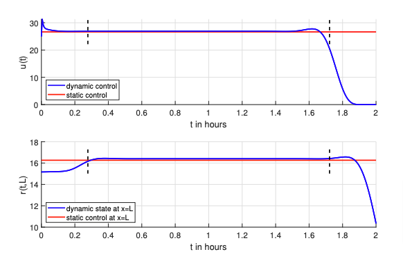
Figure 1: Optimal control (upper picture) and corresponding optimal states at x = L (lower picture).
2 Uncertain Initial Data
We consider an optimal boundary control problem with uncertain initial data given by
\left\{ \quad \begin{aligned} \min_{u \in L^2(0,T)} \quad &J_T(u) = \int_0^T f\Big( u(t) \Big) + g\Big( \mathbb{E}\big[r(t,L)\big] \Big)\ dt, \\ \text{s.t.} \quad &r(0,x) = r_{ini}^\omega(x), \\ &r_t(t,x) + c r_x(t,x) = m r(t,x), \\ &r(t,0) = u(t), \end{aligned} \right. (9)
where r_{ini}^\omega is defined by a space dependent random variable. Motivated by applications the random variable often is not completely unknown than rather given by some expected value. We model the uncertainty here by an expected deterministic state and an additional term given by a \textit{Wiener process} (W_x)_{x \geq 0} on an appropriate probability space (\Omega, \mathcal{A}, \mathbb{P}). So we have
r^\omega_{\text{ini}}(x) = r_{\text{ini}}(x) + W_x. (10)
Theorem 3
Let the assumptions (A1) and (A2) be satisfied. Then there exist optimal controls u^\delta(t) of the dynamic optimal boundary control problem (9) with uncertain data given by the Wiener process and u^\sigma of the corresponding static problem (4) that satisfy the integral turnpike property
\int_0^T \Vert u^\delta(t) - u^\sigma \Vert^2_2\ dt \leq \mathcal{C}. (11)
The time independent constant \mathcal{C} is equal to the constant in \hyperref[theorem:turnpike]{\textit{Theorem \ref*{theorem:turnpike}}}.
Corollary 4
For the expected optimal state \mathbb{E}\big[ r^\delta(t,x) \big] of the dynamic optimal control problem (9) and the corresponding optimal static state r^\sigma(x) of the static optimal control problem (4) the integral turnpike inequality
\int_0^T \Vert \mathbb{E}\big[ r^\delta(t,x) \big] - r^\sigma(x) \Vert_2^2\ dt \leq \mathcal{\tilde{C}}.
The constant \mathcal{\tilde{C}} equal to the constant in (8).
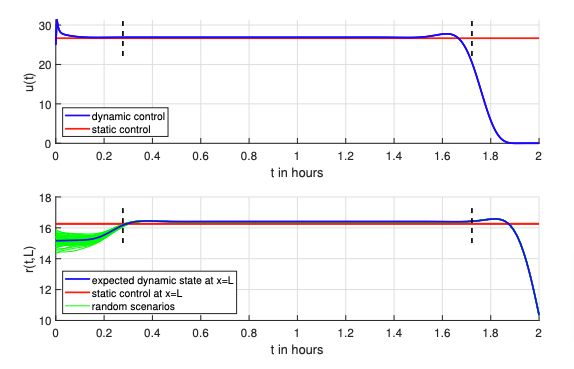
Figure 2: Optimal control (upper picture) and corresponding optimal states at x = L (lower picture).
Random Source Term
We consider uncertainty in the source term of the PDE. Consider a random variable \xi with absolutely continuous probability distribution and probability density function \varrho_\xi on an appropriate probability space (\Omega, \mathcal{A}, \mathbb{P}). Assume that \xi is integrable w.r.t. the Lebesgue-measure \lambda, i.e., the expected value of \xi exists. Let m^\omega = \xi(\omega) be a realization of the random variable. For J_T as in (2) we consider the dynamic optimal boundary control problem
\left\{ \quad \begin{aligned} \min_{u \in L^2(0,T)} \quad &J_T(u) = \int_0^T f\big(u(t)\big) + g\big( \mathbb{E}\big[ r(t,L) \big] \big)\ dt \\ \text{s.t.} \quad &r_t(t,x) + c r_x(t,x) = m^\omega\ r(t,x), \\ &r(0,x) = r_{ini}(x), \\ &r(t,0) = u(t). \end{aligned} \right. (12)
Before we state a turnpike result for the optimal boundary control problem (12) and its corresponding static problem we need to make another assumption. Define the function
e_0(t) : [0,T] \rightarrow \mathbb{R} \cup \{ \pm \infty \}, \qquad t \mapsto \int_{-\infty}^{\infty} \exp\big( z t \big)\ \varrho_\xi(z)\ dz, (13)
where \varrho_\xi is the probability density function of the random variable \xi, and define the number
e_1 := \int_{-\infty}^{\infty} \exp\bigg( z \frac{L}{c} \bigg)\ \varrho_\xi(z)\ dz. (14)
Both e_0 and e_1 are obviously positive.
• [(A3)] We assume that
e_0(t) \leq e_2 \in \mathbb{R} \lt \infty \quad \forall t \in [0,L/c], (15)
• [(A4)] We assume that
e_1 \lt \infty. (16)
Theorem 5
Let the assumptions (A1) and (A2) be satisfied. Then there \mathbb{P}-almost surely exist optimal controls u^\delta(t) of the dynamic optimal boundary control problem (12) and u^\sigma of the corresponding static problem that satisfy the integral turnpike property
\int_0^T \Vert u^\delta(t) - u^\sigma \Vert_2^2\ dt\ \leq\ \mathcal{C}_2, (17)
with a constant \mathcal{C}_2>0 that is time independent.
Lemma 6
For the expected optimal states \mathbb{E}\big[ r^\delta(t,x) \big] of (12) and \mathbb{E}\big[ r^\sigma(x) \big] of its corresponding static problem we have
\int_0^T \Vert \mathbb{E}\big[ r^\delta(t,x) \big] - \mathbb{E}\big[ r^\sigma(x) \big] \Vert_2^2\ dt \leq \mathcal{\tilde{C}}_2 (18)
The assumptions \hyperref[eq:assumption3]{(A3)} and \hyperref[eq:assumption4]{(A4)} might look strong at first glance but they basically guarantee that the expected values even exist, as it is the case for most of the common distributions.
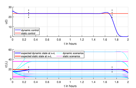
Figure 3: Optimal control (upper picture) and corresponding expected optimal state at x = L (lower picture). The lines in cyan and magenta show 10 dynamic resp. static scenarios for different values of m^\omega.
Acknowledgements
This work was supported by Deutsche Forschungsgemeinschaft (DFG) in the Collaborative Research Centre CRC/Transregio 154, Mathematical Modelling, Simulation and Optimization Using the Example of Gas Networks, Project C03, Projektnummer 239904186.
References
[1] M. Gugat, A turnpike result for convex hyperbolic optimal boundary control problems, Pure Appl. Funct. Anal., 4(4), 849–866, 2019.[2] N. Sakamoto, M. Schuster A Turnpike Result for Optimal Boundary Control Problems with the Transport Equation under Uncertainty Preprint available at https://opus4.kobv.de/opus4-trr154/frontdoor/index/index/docId/509
|| Go to the Math & Research main page


