Activation Saturation and Jacobian Attenuation in Neural Ordinary Differential Equations

Neural Ordinary Differential Equations (Neural ODEs) offer a principled way to model continuous dynamical systems with neural networks [1]. The hidden state $h(t) \in \R^d$ evolves according to

$\frac{dh}{dt} = f_\theta(h(t)), \qquad h(t_0) = h_0,$

where $f_\theta : \R^d \to \R^d$ is a multilayer perceptron with trained weights $\theta$ . Once training is finished, $\theta$ is fixed and will not change. The network no longer adapts—it defines a static vector field on the hidden state space, a dynamical system in the classical sense. The question we ask is not about learning, but about the geometry of what has been learned: what kinds of orbits can that fixed vector field support?

Most of the literature on activation functions focuses on training-time properties: does $\sigma$ help gradients flow [2, 3]? does training converge [4]? can any function be approximated [5, 6]? These are questions about what happens while the weights are being updated.
This work asks something different, a question that only becomes meaningful once training is over:

After successful training, when the weights are fixed, does a tanh-based Neural ODE retain the ability to sustain stable oscillations—or does activation saturation structurally prevent it, regardless of how well the model was trained?

The answer is quantifiably no —and the mechanism has nothing to do with training quality.

1 Where This Started

The question was raised by a companion empirical paper [7], where we trained a $\tanh$ -based Neural ODE to reproduce the dynamics of the Morris–Lecar neuron model [8], a classical biological oscillator that fires rhythmically. The behaviour was anomalous: the more we trained, the worse the oscillatory fit became. This was not a plateau—the oscillatory character was actively destroyed by further training.

Two explanations are possible. The first is a training problem: better optimisers, more data, or longer schedules might fix it. The second is structural: even after successful training, the geometry of the learned vector field may prevent stable oscillations from existing, regardless of training quality. This paper identifies a precise structural mechanism that supports the second explanation.

A natural objection is: cannot batch normalisation (BN) fix saturation? During training, BN rescales pre-activations at every step, keeping them in the active region of $\sigma$ [3]. But at inference time, BN statistics are frozen. If the model is evaluated on a trajectory that visits regions poorly represented in the training data, the pre-activations can still saturate—and no amount of post-hoc normalisation can alter this, because the weights are already fixed. The obstruction we describe is therefore genuinely an inference-time phenomenon: it can appear in a model that trained without any difficulty, and it is invisible to training diagnostics such as loss curves or gradient norms.

2 The Jacobian of the Learned Vector Field

Consider an MLP with $L$ layers,

$f_\theta(h) = W_L\,\sigma\!\left(W_{L-1}\cdots\sigma(W_1 h)\right),$

where the $W_k$ are the trained weight matrices and $\sigma$ is applied pointwise. Differentiating through the composition by the chain rule gives

$Df_\theta(h) \;=\; W_L\; \underbrace{D_{L-1}(h)}_{\text{diag}(\sigma'(a_{L-1,i}))}\; W_{L-1}\;\cdots\; \underbrace{D_1(h)}_{\text{diag}(\sigma'(a_{1,i}))}\; W_1. \qquad (2.1)$

where $a_{k,i}(h) = (W_k h_{k-1})_i$ are the pre-activations of the $k$ -th layer. Each diagonal matrix $D_k$ has entries $\sigma'$ evaluated at those pre-activations, so

$\|D_k(h)\| \;=\; \max_i |\sigma'(a_{k,i}(h))|.$

By submultiplicativity of the operator norm,

$\|Df_\theta(h)\| \;\le\; \prod_{\ell=1}^{L} \|W_\ell\| \;\cdot\; \prod_{k=1}^{L-1} \|D_k(h)\|.$

The central observation is elementary: if $\sigma'$ is small at the pre-activations of some hidden layers, those $D_k$ matrices suppress the entire product. Everything in the paper is a consequence of this single fact.

3 Theorem 1: Jacobian Attenuation

Definition 3.1.
Let $U \subset \R^d$ be a convex open set. We say that $q$ hidden layers are $\delta$ -saturated on $U$ if $\max_i |\sigma'(a_{k,i}(h))| \le \delta$ for all $h \in U$ , for $q$ values of $k \in \{1, \ldots, L-1\}$ .
Set $\Lambda_\sigma := \sup_{x \in \R} |\sigma'(x)|$ (for $\tanh$ : $\Lambda_\sigma = 1$ ), and let

$C_W \;:=\; \prod_{\ell=1}^{L} \|W_\ell\| \cdot \Lambda_\sigma^{L-1-q}.$

Theorem 3.1 (Jacobian Attenuation). If $q$ hidden layers are $\delta$ -saturated on $U$ , then

$\|Df_\theta(h)\| \;\le\; C_W\,\delta^{\,q} \qquad \forall\, h \in U. \qquad (3.1)$

The bound is uniform over all $h \in U$ and is an intrinsic property of the trained model—it does not depend on how $\theta$ was obtained.
Since $\delta^q$ decays exponentially in the saturation depth $q$ , the suppression can be dramatic: three layers with $\delta = 0.1$ give a factor of $10^{-3}$ .

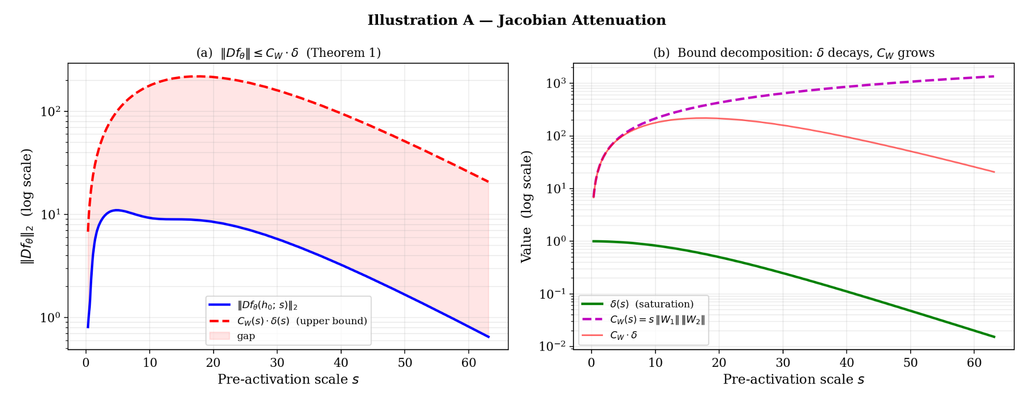
Illustration of Theorem 1. A two-layer $\tanh$ MLP (32 hidden units) is trained on the Stuart-Landau vector field; the weights are then frozen and a pre-activation scale $s$ is varied to control saturation.
Left: actual spectral norm $\|Df_\theta\|_2$ (blue) versus the theoretical upper bound $C_W\,\delta(s)$ (red dashed); the bound holds for all $s$ .
Right: $\delta(s)$ decays exponentially (green) while $C_W(s)$ grows only linearly (pink); their product still goes to zero.

4 The Floquet-Liouville Obstruction

4.1. The Liouville-Abel-Jacobi identity
We now connect the small Jacobian to the stability of periodic orbits via a classical identity from ODE theory [9, 10].
For any periodic orbit $\gamma$ of period $T$ ,

$\det M_\gamma \;=\; \exp\!\left(\int_0^T \text{Tr}\!\left(Df_\theta(\gamma(t))\right) dt\right) \;=\; \exp\!\left(\int_0^T \mathrm{div}(f_\theta)(\gamma(t))\,dt\right). \qquad (4.1)$

where $M_\gamma$ is the monodromy matrix of $\gamma$ , which measures how a small displacement from $\gamma$ grows or shrinks after one complete period.
Attraction requires $\det M_\gamma \lt 1$ (this is exact for $d=2$ ; a necessary condition for $d > 2$ ). For the Stuart–Landau oscillator used as our benchmark, $\det M_\gamma = e^{-4\pi} \approx 3.5 \times 10^{-6}$ –strongly dissipative.

Since $\mathrm{div}(f_\theta) = \text{Tr}(Df_\theta)$ and $|\text{Tr}(A)| \le d\, \|A\|$ for any $d \times d$ matrix [11], Theorem 1 gives $|\mathrm{div}(f_\theta)| \le d\,C_W\,\delta^q$ uniformly on $U$ , and substituting into (4.1) immediately yields the following result.

4.2. Theorem 2: Floquet-Liouville Obstruction

Theorem 4.1.
Under the hypotheses of Theorem 1, if $\gamma$ is a periodic orbit of period $T$ contained in $U$ , then

$e^{-d\,C_W\delta^q T} \;\le\; \det M_\gamma \;\le\; e^{+d\,C_W\delta^q T}. \qquad (4.2)$

As $\delta \to 0$ (deeper saturation), $\det M_\gamma \to 1$ , and the orbit ceases to attract.

The theorem does not forbid periodic orbits –it forbids them from being strongly attracting. If $d\,C_W\delta^q T \lt \eta$ , no orbit in $U$ can attract at contraction rate $\eta$ or higher.
The structural tension is precise: dissipative oscillators require $\det M_\gamma \ll 1$ , while saturation forces $\det M_\gamma \to 1$ , making the vector field effectively volume-preserving in the saturated region.

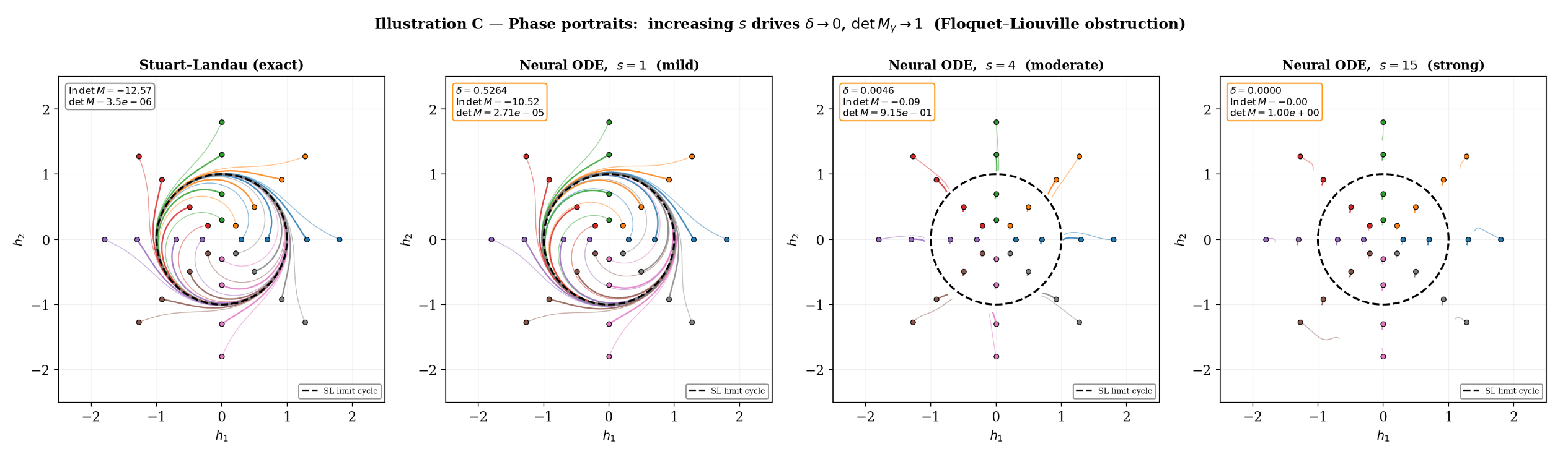
Illustration of Theorem 2. Phase portraits of a bias-shifted $\tanh$ Neural ODE (256 hidden units) trained on the Stuart–Landau oscillator, at increasing saturation scales $s \in \{1, 4, 15\}$ .
At $s = 1$ (mild saturation): $\det M \approx 10^{-5}$ , trajectories spiral toward the limit cycle from both sides.
At $s = 4$ : $\det M \approx 0.91$ , contraction is nearly gone.
At $s = 15$ : $\det M = 1.00$ to four decimal places, the flow is conservative and the limit cycle ceases to attract.

4.3. Converse: non-saturating activations can sustain stable oscillations
The obstruction is not universal. For non-saturating activation functions—the prime example being SiLU ( $\sigma(x) = x/(1+e^{-x})$ ), whose derivative approaches $1$ for large positive inputs –the diagonal matrices $D_k$ stay bounded away from zero, and the chain leading to (4.2) breaks at the first step. Using the $C^1$ universal approximation theorem [5] and a structural stability argument [10], one can show that a SiLU-based Neural ODE can sustain a strongly attracting limit cycle. The implication for practitioners is direct: for oscillatory modelling tasks, the choice of activation function is not a hyperparameter –it determines whether the model can represent the target dynamics at inference time.

The complete five-step argument is:

$\underbrace{|\sigma'| \le \delta}_{\text{saturation}} \;\xRightarrow{\text{Thm.\,1}}\; \underbrace{ \|Df_\theta\| \le C_W\delta^q}_{\text{Jacobian attenuation}} \;\Rightarrow\; \underbrace{|\mathrm{div}(f_\theta)| \approx 0}_{\text{trace bound}} \;\xRightarrow{\text{Liouville}}\; \underbrace{\det M_\gamma \to 1}_{\text{no strong attraction.}}$

5 Further Research

Several natural questions remain open.

Higher dimensions. For $d = 2$ , the monodromy matrix has a single transverse eigenvalue and $\det M_\gamma$ controls orbital stability exactly. For $d > 2$ (e.g.\ the four-dimensional Hodgkin–Huxley model [12]), $\det M_\gamma$ is only the product of all Floquet multipliers; a refinement that controls individual multipliers is needed.

Weight growth during training. Theorem 1 assumes $C_W$ is bounded. Whether gradient-based optimisers increase weight norms to compensate for small $\delta$ at stationary points of the training loss—and whether the product $C_W\,\delta^q$ remains bounded or not—is an open question requiring tools from optimisation theory.

Adaptive activations. If $\sigma(x) = \tanh(\beta x)$ with a trainable $\beta$ , the obstruction applies whenever $\beta$ is large enough to saturate the relevant pre-activations. Whether training reliably avoids this, or inadvertently deepens it, is open.

Homoclinic extension. Theorem 2 requires a periodic orbit of finite period $T$ ; as $T \to \infty$ the bound becomes vacuous. An entirely different analysis—drawing on Shilnikov conditions or Melnikov-type perturbation theory—is needed for homoclinic orbits, which is precisely the regime of the Morris–Lecar failure that originally motivated this work.

A central conjecture ties these directions together: the local derivative profile of $\sigma$ is a more fundamental determinant of dynamical expressibility in Neural ODEs than the global Lipschitz constant of $f_\theta$ . If true, this reframes activation selection for time-series modelling as a question of dynamical geometry rather than optimisation convenience.

References

The results presented here are part of a manuscript in preparation.
A preprint is available at https://cris.fau.de/publications/361846623/ (arXiv:2604.00543)
[1] R. T. Q. Chen, Y. Rubanova, J. Bettencourt, and D. Duvenaud. Neural ordinary differential equations. NeurIPS, 2018. arXiv:1806.07366.
[2] X. Glorot and Y. Bengio. Understanding the diﬀiculty of training deep feedforward neural networks. AISTATS, 2010.
[3] S. Ioffe and C. Szegedy. Batch normalization: Accelerating deep network training by reducing internal covariate shift. ICML, 2015. arXiv:1502.03167.
[4] Z. Gao, M. Shi, and S. Du. Global convergence of deep networks with one wide layer followed by pyramidal topology. ICLR, 2025.
[5] K. Hornik, M. Stinchcombe, and H. White. Multilayer feedforward networks are universal approximators. Neural Networks, 2(5):359–366, 1989. doi:10.1016/0893-6080(89)90020-8.
[6] G. Cybenko. Approximation by superpositions of a sigmoidal function. Mathematics of Control, Signals and Systems, 2(4):303–314, 1989. doi:10.1007/BF02551274.
[7] N. Matzakos and C. Sfyrakis. Comparing physics-informed and neural ODE approaches for modeling nonlinear biological systems: A case study based on the Morris–Lecar model.arXiv preprint, 2026. arXiv:2603.26921.
[8] C. Morris and H. Lecar. Voltage oscillations in the barnacle giant muscle fiber. Biophysical Journal, 35(1):193–213, 1981. doi:10.1016/S0006-3495(81)84782-0.
[9] E. A. Coddington and N. Levinson. Theory of Ordinary Differential Equations. McGrawHill, 1955.
[10] C. Chicone. Ordinary Differential Equations with Applications. Springer, 2006. doi:10.1007/0387-35794-7.
[11] R. A. Horn and C. R. Johnson. Matrix Analysis, 2nd ed. Cambridge University Press, 2013.
[12] A. L. Hodgkin and A. F. Huxley. A quantitative description of membrane current and its application to conduction and excitation in nerve. Journal of Physiology, 117(4):500–544, 1952. doi:10.1113/jphysiol.1952.sp004764.