
Nonlinear hyperbolic systems: Modeling, controllabiliy and applications
The control theory of hyperbolic systems is an important topic in continuum and fluid mechanics. Networks of nonlinear hyperbolic systems arise in real world applications, e.g. planar or out-of-plane networks of vibrating strings, shearable beams, gas networks and shallow water systems. On these typical 1d hyperbolic networks, the mathematical modeling and particularly the interface or transmission conditions along with the corresponding controllability properties are the focus of this post.
Modeling: 1d Nonlinear hyperbolic systems
We consider the state function given by the general 1-D nonlinear hyperbolic systems located on [0, L] :
y_{t}+ A(y)y_{x}=F(y), \quad t\ge 0, 0\le x\le L (1)
where
- y= (y_1,\cdots, y_n)^T is a vector function of (t,x),
- A(u) has n distinct non-vanishing real eigenvalues \lambda_i(y) and a complete set of left (resp. right) eigenvectors l_i(y) = (l_{i1}(y),..., l_{in}(y)) (resp. r_i(y) = (r_{1i}(y),...,l_{ni}(y))^T) (i= 1,...,n).
- After a linear change of variables, we may assume l_{ij}(0)=\delta_{ij}(i,j=1,...,n), where \delta_{ij} stands for the Kronecker symbol.
- F(y)= (f_1(y),...,f_n(y))^T is a given vector function of y with F(0)=0.
For simplicity, the eigenvalues of A(0), which is a diagonal matrix, are ordered , i.e.
\lambda_1(0) \lt \lambda_2(0) \lt \cdots \lt \lambda_m(0) \lt 0 \lt \lambda_{m+1}(0) \lt \cdots \lt \lambda_n(0)
The boundary conditions are given as follows:
x=0: y_s= G_s(t, y_1, ..., y_m) + u_s(t) \quad (s=m+1,..., n), (2)
x=L: y_r= G_r(t, y_{m+1}, ..., y_n) + u_r(t) \quad (r=1,..., m), (3)
where G_i(i = 1, \cdots, n) and u_i (i = 1, \cdots, n) are C^1 functions satisfying
G_i(t, 0,\cdots, 0)\equiv 0 \quad (i=1,...,n).
(2) and (3) are the most general nonlinear boundary conditions to guarantee the well-posedness for the forward mixed problem.
On the domain \{(t,x)| t\ge 0, 0\le x\le L\} we consider the forward mixed initial-boundary value problem for system (1) with the the initial condition
t=0:~ y=y_0(x), \quad 0\le x\le L. (4)
We always suppose that the conditions of C^1 compatibility are satisfied at the point (t,x)=(0,0) and (0,L), respectively, then the forward mixed problem (1), (2) – (3) and (4) at least admits a unique C^1 solution y=y(t,x) locally in time.
Many physical models are governed by this general model, for example: the telegrapher equations (Heaviside, O. (1892)), the Saint-Venant equations (Barre de Saint-Venant (1871)), the Saint-Venant-Exner equations (Hudson-Sweby (2003)), Heat exchangers (G.Bastin-JMC (2015)).
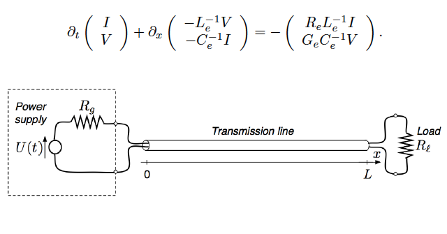
Figure 1. The telegrapher equations (Heaviside, O. (1892))
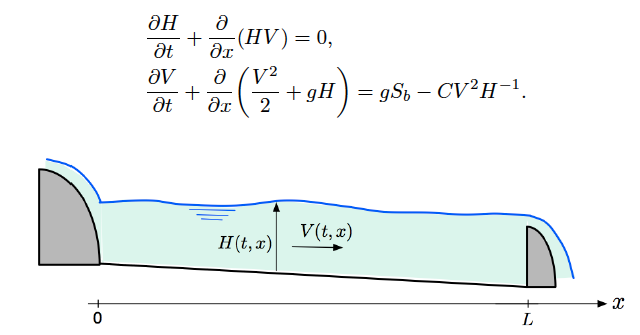
Figure 2. The Saint-Venant equations (Barre de Saint-Venant (1871))
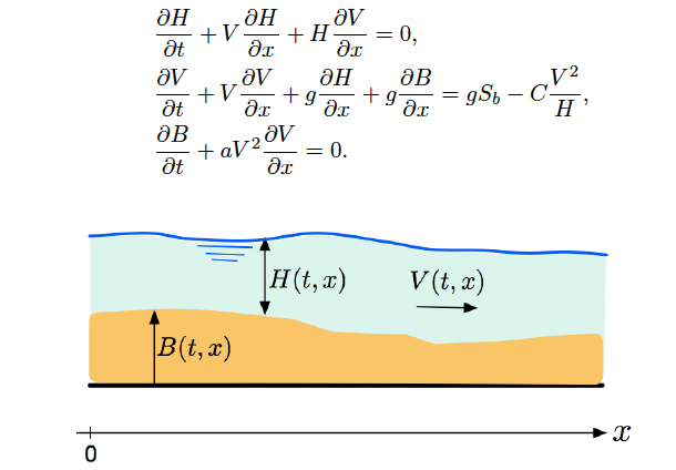
Figure 3. The Saint-Venant-Exner equations (Hudson-Sweby (2003))
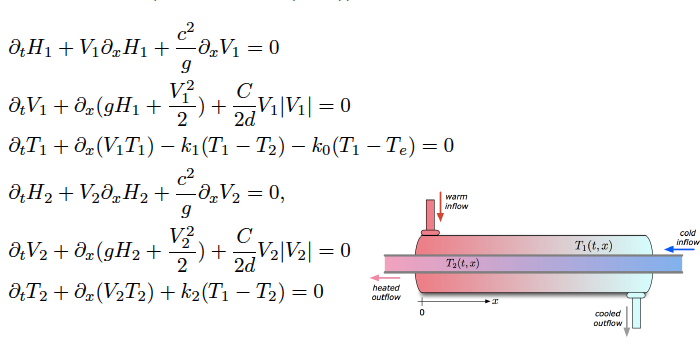
Figure 4. Heat exchangers (G.Bastin-JMC (2015))
Control problems
Different control problems may be addressed depending on how the control objective is formulated, such as controllability, observation, optimal control, stabilization and feedback control. For the boundary controllability, roughly speaking the goal is applying suitable boundary control u(t) to drive exactly the state y to the prescribed one y_d, such as:
Null boundary controllability (NBC) problem
Let T>0. For any given \phi: [0,L] \to \mathbb{R}^n. Does there exist boundary controls at (2) or/and (3) such that the solution of the control system satisfies (4) and
y(T,x) =0, x\in [0,L]. (5)
Since the hyperbolic wave has a finite speed of propagation, in order to get the exact boundary controllability, T should be suitably large.
Exact boundary controllability (EBC) problem
The final state (5) is reduced by
y(T,x) =y_{d}(x), x\in [0,L], (6)
in which y_d is arbitrarily chosen in an appropriate space. We call it a local controllability if y_0 and y_d are close to the equilibrium point.
The null/exact boundary controllability (NBC/EBC) of linear hyperbolic systems was obtained in a complete manner by the work of D. L. Russel (1978) and J.-L Lions (1988). Furthermore, quite mature and plentiful mathematical tools, e.g. Hilbert uniqueness method, duality method, Fourier series, multiplier have been developed in semi- linear wave equations by the work of E. Zuazua (1990,1993), O. Y. Emanuilov (1989), I. Lasiecka (1991) etc. For quasilinear case, the local null/exact controllability are obtained by T.T. Li, B.Y. Zhang (1998, 2002, 2003, 2010) and B.P.Rao (2010).
Another important controllability problem has been proposed in recent years according to practical application requirements:
Exact boundary controllability of nodal profile (NP-EBC) problem
Let T > T_0 > 0. Does there exist boundary controls such that (a part of) the boundary traces of state fit to a given profile on a node after after a suitably long time T_0, e.g. the state at x = 0 satisfies
y(t,0) = y_d(t),∀t ∈ [T_0,T].
This kind of nodal control problem was first introduced by M. Gugat, M. Herty and V. Schleper [1] motivated by the real-world gas networks, to meet the given customer demand in density and flux by a compressor control.
Main Results: boundary controllability
In control theory, the following essential issues in the context of controllability properties of nonlinear hyperbolic systems are addressed:
- the optimal controllability time
- the minimum number of required controls
In the following, we give two important results for EBC and NP-EBC of general quasilinear hyperbolic systems (1). And these mathematical results could be applied and extended to complex networks arising in real world, and also give a kind of control design to determine the location and required evolution of control function. See more details in books [2] and [3].
Main result 1 [EBC]. In one-sided control case (only m controls u_1, ..., u_m acts on x = L), in a neighbourhood of an equilibrium (around 0), the system (1), (2)-(3) and (4) is locally exact boundary controllable provided by the following three conditions (A1-A3):
(A1) n-m\le m,
(A2) in a neighborhood of y=0 the (2) satisfies
y_s =G_s(t, y_1,...y_m) + u_s(t) (s=m+1,...,n)
\Longleftrightarrow y_{\bar r} =\overline G_{\bar r}(t, y_{n-m+1},...y_m, y_{m+1},...y_{n}) + \overline u_{{\bar r}}(t) (\bar r= 1,...,n-m),
(A3) T> L ( \frac{1}{|\lambda_m(0)|} + \frac{1}{|\lambda_{m+1}(0)|}).
To be specific, for any given boundary data u_s (t) with small C^1[0,T] norm, satisfying the conditions of C^1 compatibility at the points (t,x) = (0,0) and (T, L), respectively, there exist m boundary controls u_r (r=1,..,m), such that the corresponding mixed problem (1), (2)-(3) and (4) admits a unique semi-global C^1 solution y=y(t,x) with small C^1 norm on the domain \mathcal R(T) = \{(t,x)| 0\le t\le T, 0\le x\le L\} , which verifies exactly the final condition (6). See in Figure 5.
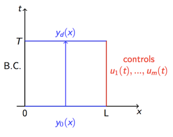
Figure 5. One-sided exact boundary controllability
Furthermore, (A1-A3) answer the two questions addressed at the beginning of this section. For one-side controllability, we need (A1) enough controls, (A2) coupling conditions on the non-control side, and (A3) sufficient time for controls.
Main result 2 [NP-EBC]. Let T_0 \gt \frac{L}{\lambda_m(0)} and T>T_0. In a neighbourhood of an equilibrium (around 0), the system (1), (2)-(3) and (4) is local boundary controllability of nodal profile.
To be specific, for any given initial data y_0(x), nodal profile y_d and boundary functions u_s (s=m+1, ..., n) with small C^1 norm, satisfying the conditions of C^1 compatibility at the point (t,x)=(0,0), then there exist m boundary controls u_r (r=1,...,m) on the other side x=0, such that the corresponding mixed problem (1), (2)-(3) and (4) admits a unique semi-global C^1 solution y=y(t,x) with small C^1 norm on the domain \mathcal R(T) = \{(t,x)| 0\le t\le T, 0\le x\le L\}, which fits exactly the given value y_d(t) on the boundary node x=0 for t\in [T_0,T].
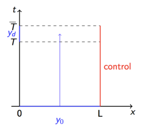
Figure 6. Exact boundary controllability of nodal profile
Both Result 1 and Results 2 can be proved by the constructive method with modular structure introduced by Tatsien Li. Very recently, these results and method are generalized and applied on nonlinear string networks and other hyperbolic systems – which are governed by meaningful physical model and reasonable interface conditions.
Applications and expansion
For the following nonlinear hyperbolic systems, a simple and efficient constructive method with modular structure has been suggested by us in recent years to get the exact boundary controllability and of nodal profile in one-space-dimensional case. Another challenge here is to find physically meaningful interface conditions that lead to a wellposed (nonlinear) systems, (see in Figures 7-10) that can have complex dynamics at the interface or a complex network structure, e.g. a loop. After that the control design is addressed, both from a theoretical and numerical perspective.
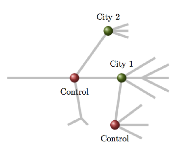
Figure 7. Flow control on gas network
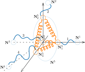
Figure 8. Coupling strings via Hookean body
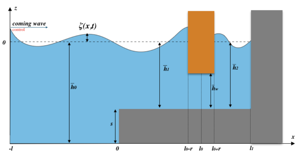
Figure 9. Shallow water system with an obstacle
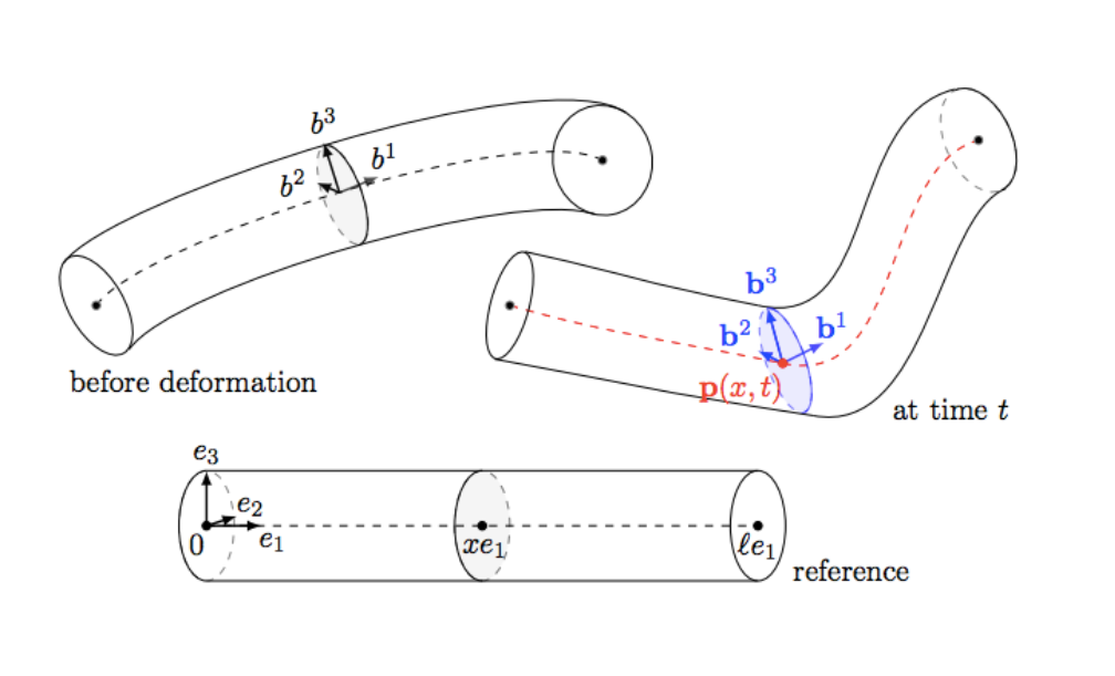
Figure 10. Geometrically exact beams
Flow control on gas network
A wide-mentioned application of NP-EBC is the gas network modeled by one dimensional isothermal Euler equa- tions [1]. For a single pipe, the system is given by a hyperbolic balance law:
\rho_t+q_x=0,\quad q_t+(\frac{q^2}{\rho}+a^2\rho)_x = -f_g \frac{q|q|}{2D\rho}, (7)
where \rho(t, x) is the density of the gas, q(t, x) is the flux in the pipe, and f_g is the friction factor, D is the diameter of the pipe.
In real–world gas networks the pressure P=a^2\rho (with constant a) along a pipe decreases due to strong friction effects. So we always need to place a compressor station to increase the pressure P of a gas flow q from P_{in} to p_{out}. The dynamics of the compressor at x=0 connecting two pipes is given as
q^{(1)}(t,0)= q^{(2)}(t,0),\quad u(t) =q^2(t,0)\left((\frac{\rho^{(2)}(t,0}{\rho^{(1)}(t,0)})^\kappa-1\right), (8)
where \kappa=(\gamma-1)/\gamma with \gamma the isentropic coefficient of the gas. And u(t,x) as the control function is proportional to the applied compressor power P.
In [1] the authors find control u to drive the solutions on certain network in order that the given customer demand (\rho_B(t), q_B(t)) in density and flux is fulfilled exactly for all time t\in[t^*,T_0] with given t^*> T_0>0:
(\rho^{(2)}, q^{(2)})\Big|_{x=L_2} = (\rho_B(t), q_B(t)), \quad \forall t\in [t^*,T_0]. (9)
Network of vibrating strings with spring and masses
When we encounter more complex coupling situations, such as non-local dynamic boundary conditions, it is still feasible to use constructive methods to achieve the corresponding EBC and NP-EBC for vibrating string networks.
We consider networks of elastic strings with end masses, where the coupling is modelled via elastic springs. The model is given by representative of a network of nonlinear strings, which the strings are coupled to elastic bodies. The motion of i-string(i = 1,...N) is denoted by \mathbf{y^i}(t, x), a vector function in \mathbb R^3. In the usual way, we have the following system of non-linear wave equations:
\rho_i \mathbf{y}^i_{tt}(x,t) = [\mathbf{G}^i(\mathbf{y}^i_x(x,t))]_x -\rho_i g \mathbf{e}, (10)
with \mathbf{G}^i:\mathbb R^3\mapsto \mathbb R^3 defined in form \mathbf{G}^i(\mathbf{v}) := V^i_s(|\mathbf{v}|)\frac{\mathbf{v}}{|\mathbf{v}|}. \mathbf{e} is the vertical unit vector and g is the gravitational constant.
Next, for index i,j at the Hookean body (reduced by spring and mass), there is no continuity condition across the joints, we are led to the multiple nodal condition
\epsilon_{i}\mathbf{G}^i(\mathbf{y}^i_x(x_{i},t))+m_i\mathbf{y}^{i}_{tt}(x_{i},t) + \sum\limits_{i \in \mathcal{J}_i} \kappa_{ij}( \mathbf{y}^{j}(y_{i},t)-\mathbf{y}^{i}(x_{i},t))=0, (11)
where \epsilon_{i}=\pm 1, the last term stands for the spring stiffness terms. The coupled system (10)-(11) tends to the classical string network model with Kirchhoff and continuity transmission conditions, as the spring stiffness terms \kappa_{ij} tend to the infinity and the masses m_i at the nodes vanish. Due to the presence of point masses at the nodes, boundary conditions become dynamical and, consequently, the corresponding first order system of quasilinear balance laws exhibits nonlocal boundary conditions.
Without essential difficulty, the EBC and NP-EBC results can be extended to this kind of string network in a neighbor of stretched equilibrium. The initial work for coupled strings via spring is at [4], the modeling and controllability for networks of strings without springs is at [5].
Shallow water system with an obstacle
Another example is one dimensional nonlinear shallow water system, describing the free surface flow of water as well as the flow under a fixed gate structure (see the figure of the shallow water system with an obstacle above). The motion of the fluid is governed by the 1d nonlinear shallow water equations:
\partial_t\zeta+\partial _xq=0, \quad \partial_t q+\partial_x \left(q^2/h\right)+gh\partial_x \zeta=0, (12)
where \zeta(t, x) is the free surface elevation, h(t, x) is the fluid height, and q(t,x) is the horizontal discharge. In this situation, we can use a ‘chain-like network’ consisting of 3 parts (0,1,2). Part 1 represents the region to the left (x<0), part 2 is the more shallow region to the left of the obstacle (0 < x < l_0-r), and part 3 is the (more shallow) region to the right of the obstacle (l_0 + r < x < l_1).
The transmission conditions are as follows
x=0:\quad \zeta_0(t,0)=\zeta_1(t,0),\quad q_0(t,0)=q_1(t,0), (13)
x= l_0\pm r:\quad q_2(t, l_0+r) =q_1(t, l_0-r)= q_w(t), \quad \Big[\frac{q_i^2}{2h_i^2}+g\zeta_i\Big]_{i=1, x=l_0-r}^{i=2,x=l_0+r}=-\alpha \frac{\mathrm d}{\mathrm dt} q_w(t), (14)
where \alpha= 2r/h_w, and the subscripts are used to indicate the corresponding interval.
The resulting system of partial differential equations with several transmission conditions (13)-(14) is a simplified model of a wave energy converter. The problem setting naturally leads us to study the EBC in a prescribed region. In particular, we use the concept of NP-EBC in which at a given node, time-dependent profiles need to be reached by means of boundary controls. By rewriting the system into a hyperbolic system with nonlocal boundary conditions, we at first establish the semi-global classical solutions of the system, then get the local controllability, and finally the required controls using a constructive method. The constructive method provides a practical algorithm to calculate the required boundary control function. See more details at [6].
Geometrically exact beams
The last extension of the work is given on networks of shearable beams that may undergo large motions — another type of important physical model, which results in a quasilinear model. The quasilinear system can be reduced to a 1st Order Semilinear IGEB model by a nonlinear transformation. You can find the modeling in “Control and Stabilization of Geometrically Exact Beams“.
Here a specific network with a cycle was considered (see below Figure 11). So far, we have proved that it is possible to realize the NP-EBC with the idea of cut-off method. This is the first result we know for this kind of network. We can foresee that, the corresponding NP-EBC is also reasonable on general networks, furthermore, the explicit method encourages us to give a numerical algorithm to show the control. See more details at [7].
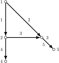
Figure 11. A network with a cycle
Main post image credits: J. Spillmann and M. Teschner, “Cosserat Nets,” in IEEE Transactions on Visualization and Computer Graphics, vol. 15, no. 2, pp. 325-338, March-April 2009, doi: 10.1109/TVCG.2008.102.
References
[1] M. Gugat, M. Herty, V. Schleper, Flow control in gas networks: Exact controllability to a given demand, Math. Meth. Appl. Sci., 34(7)(2011), 745-757.
[2] T.T. Li, Controllability and Observability for Quasilinear Hyperbolic Systems, AIMS Series on Applied Mathematics, vol. 3. AIMS & Higher Education Press, 2010.
[3] T.T. Li, K. Wang, Q.L.Gu, Exact Boundary Controllability of Nodal Profile for Quasilinear Hyperbolic Systems, Springer Briefs in Mathematics, Springer, 2016.
[4] Y. Wang, G. Leugering, T. Li, Exact boundary controllability for a coupled system of quasilinear wave equations with dynamical boundary conditions, Nonlinear Analysis: Real World Applications. 49 (2019), 71-79.
[5] Y. Wang, T.Li, Exact boundary controllability of partial nodal profile for network of strings, Nonlinear Analysis: Real World Applications, 62 (2021), https://doi.org/10.1016/j.nonrwa.2021.103383.
[6] G. Vergara-Hermosilla, G. Leugering, Y. Wang, Boundary Controllability of a System Modeling a Partially Immersed Obstacle, Control, Optimisation and Calculus of Variations, 27 (2021).
[7] G. Leugering, C. Rodriguez, Y. Wang, Nodal Profile Control For Networks Of Geometrically Exact Beams, Journal de Mathématiques Pures et Appliquées, doi:10.1016/j.matpur.2021.07.007, 2021.
|| Go to the Math & Research main page


