
Neural ODEs for interpolation and transport: From tight to shallow

Introduction
We consider in our work residual neural networks (ResNets) which take the form
\mathbf{x}_{k+1}=\mathbf{x}_k+\sum_{i=1}^p \textbf{w}^k_i\sigma\left( \textbf{a}^k_i \mathbf{x}_k+b^k_i\right), \qquad k \in\{0, \ldots, M-1\}, (1.1)
for some initial input \mathbf{x}_0\in \mathbb{R}^d. The states \mathbf{x}_k \in \mathbb{R}^d are the output after each layers, with \textbf{x}_{M} being the final output. The depth of the neural network is the number of layers M, and the width is the number of neurons p\geq1. The parameters (\textbf{a}_k^i,\textbf{w}_k^ib_k^i)_{ik}\subset(\R^d\times\R^d\times\R)^{M\times p} are optimizable weights. The function \sigma:z\in\R\longmapsto\R is a fixed Lipschitz-continuous nonlinearity called the activation function. Throughout this work we will use the Rectified Linear Unit \sigma(z)=\max\{z,0\}.
It has recently been observed [17, 11, 2, 3] that ResNets can be interpreted as the forward Euler discretization scheme for the so-called neural ordinary differential equation (NODE):
\text{\.{\textbf{x}}}=\sum_{i=1}^p \textbf{w}_i(t)\sigma(\textbf{a}_i(t)\cdot\textbf{x}+b_i(t)), (1.2)
where (\textbf{w}_i,\textbf{a}_i,b_i)_{i=1}^p\in L^\infty(\R^d\times\R^d\times\R)^p are the control variables.
It is common to take the controls as piecewise constant in time. This allows to interpret each of the constant parts as a layer.
This new formulation allows us to use the well established tools of the mathematical theory of dynamical systems and control to understand neural networks and exhibit theoretical guarantees.
In this context, the classical paradigms of interpolation and universal approximation in neural networks can be recast as a problem of approximated or exact control, as studied in [4, 9, 13, 15]. In addition, the training process of the network translates as an optimal control problem [1, 7 , 8]. Other works rigorously establish the continuous formulation (1.2) with its corresponding optimal control problem as a mean-field limit of the training problem with the discrete formulation (1.1), see for example [6, 10, 12].
Two extreme models can be formulated:
• Shallow NODEs (SNODEs), which correspond to one-layer neural networks (see Figure 1a), are obtained when the controls are time-independent and the equation is autonomous:
\text{\.{\textbf{x}}}=\sum_{i=1}^p \textbf{w}_i\sigma\left( \textbf{a}_i\cdot\textbf{x}+b_i\right). (1.3)
These architectures are very popular in the scientific communities, particularly because they enjoy important theoretical proprieties (see for example [5]). However, we often have no explicit methods as to how to construct the weights (\textbf{w}_i,\textbf{a}_i,b_i)_{i=1}^p and try instead to solve a cost-optimization problem.
• Tight NODEs (TNODEs), which correspond to deep neural networks with one-neuron width (see Figure 1b), are obtained when p=1:
\text{\.{\textbf{x}}}= \textbf{w}(t)\sigma\left(\textbf{a}(t)\cdot\textbf{x}+b(t)\right) (1.4)
With this architecture, designing constructive method to perform various tasks is easier and the constructions are natural. In [13] and [14], the authors give an explicit construction of the controls to perform tasks of interpolation, approximation and transport. However, these one-neuron width architecture is very unusual and rarely considered in practice.
A representation of these two architectures is given by Figure 1, where F=\sum_{i=1}^p \textbf{w}_i\sigma(\textbf{a}_i\cdot\textbf{w}+b_i) for Figure 1a and F(\textbf{x})=\textbf{w}\sigma(\textbf{a}\cdot\textbf{w}+b) for Figure 1b.
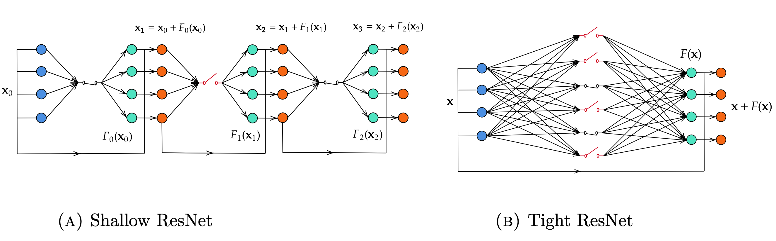
Figure 1. Tight ResNet
In this context, the classical paradigms of interpolation and universal approximation can be recast from a control perspective, as studied in [4, 9, 13, 15]. In addition, the training process of the network may be translated as an optimal control problem [1, 7, 8]. Other works rigorously establish the control problem in the continuous formulation (1.2) as a mean-field limit of the discrete counterpart (1.2) [6, 10, 12].
With these architecture, designing constructive method to perform various tasks is easier and the constructions are natural. In [14] and [13] the authors give an explicit construction of the controls to perform tasks of interpolation, approximation and transport. However, these one-neuron width architecture is very unusual and rarely considered in practice.
The goal of our work is to try to build a constructive theory encompassing both the Shallow and Tight models. This would allow to enjoy both the theoretical guarantees of the Shallow models (1.3) and the constructive and explicit methods used for the Tight models (1.4).
2. Main results
2.1. Interpolation/Simultanuous Control
Let d\geq 2 and consider a dataset containing N pairs of distinct points
\mathcal{SS}=\{(\textbf{x}_n,\textbf{y}_n)\}_{n=1}^N\subset\R^d\times\R^d. (2.1)
Our goal is to classify the input points \{\textbf{x}_n\}_{n=1}^N based on their corresponding labels \{\textbf{y}_n\}_{n=1}^N. This objective can be reformulated as a simultaneous control problem: find controls (\textbf{w}_i,\textbf{a}_i,b)_{i=1}^p\in L^\infty(\R^d\times\R^\times\R)^p such that the associated flow of the Neural ODE (1.2), \phi_T(.;\textbf{w},\textbf{a},\textbf{b}), interpolate the dataset \mathcal{SS}:
\phi_T(\textbf{x}_n;W,A,\textbf{b})=\textbf{y}_n,\qquad \text{ for all }n=1,\dots,N. (2.2)
where \textbf{w}=(\textbf{w}_1,\dots,\textbf{w}_p),\textbf{a}=(\textbf{a}_1,\dots,\textbf{a}_p),\textbf{b}=(b_1,\dots,b_p). Notice that by the uniqueness of solutions of the Cauchy problem, we have to impose that the targets \{y_n\}_{n=1}^N are distinct.
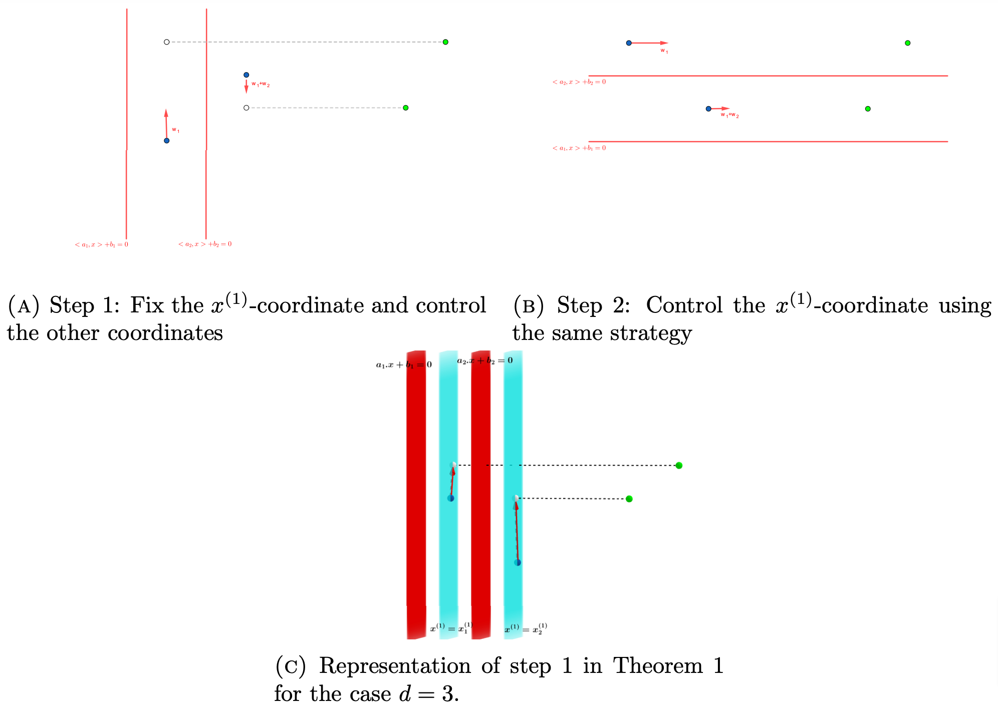
Figure 2. Qualitative representation of the proof of theorem 1.
Theorem 1. Simultaneous Control with p neurons
Consider the system (1.2) with d\geq2, a dataset \mathcal{SS}=\{(\textbf{x}_n,\textbf{y}_x)\}_{n=1}^N\subset\R^d\times\R^d with distinct targets \{\textbf{y}_i\}_{i=1}^N, and let T>0 be fixed.
For any p\geq1, there exist controls \left(\textbf{w}_i,\textbf{a}_i,b_i\right)_{i=1}^p\subset L^\infty\left((0,T);\R^d\times\R^d\times\R\right) such that the flow \phi_T(\cdot;W,A,\textbf{b}) generated by (1.2) satisfies:
\phi_T(\textbf{x}_n;W,A,\textbf{b})=\textbf{y}_n,\qquad \text{ for all }n=1,\dots,N.
Moreover, the controls are piecewise constant and the number of discontinuities is:
M=2\left\lfloor\frac{N}{p} \right\rfloor+1.
A qualitative representation of the construction of the required controls is shown in Figures 2.
We notice how the number of time-discontinuities of the piecewise constant controls (i.e the number of layers) decreases as the number of neurons p increases. This means that as p grows from p=1 to larger values, we transition from the Tight model (1.4) to an architecture more similar to (1.3).
2.2. Neural Transport
So far we considered the system (1.2) with points as initial data. We next consider the case where the position of the initial data is not certain and is rather described by a probability measure \rho_0 on \R^d.
The problem thus becomes to control the equation so that it drives an initial Borel probability \rho_0 to a target Borel probability \rho_*, in the sense of finding controls (\textbf{w}_i,\textbf{a}_i, b_i)_{i=1}^p\in L^\infty(\R^d\times\R^d\times\R)^p such that:
W_1(\phi_T(\cdot;\textbf{w},\textbf{a},\textbf{b})\#\rho_0,\rho_*)\leq\epsilon,
where we used the Wasserstein-1 distance (see [16]) and f\#\mu is the push-forward of \mu by the function f.
This question can be recast as a control problem for a transport equation. Indeed, if we define the measure valued path \rho(t)=\phi_t\#\rho_0, where \phi_t is the flow associated with (1.2), then \rho(.) satisfies the neural transport equation:
\begin{cases} \partial_t \rho &+ div_\textbf{x}\left(\left(\sum_{i=1}^p \textbf{w}_i\,\sigma(\textbf{a}_i\cdot\textbf{x}+b_i)\right)\rho\right)=0\\ \rho(0)&=\rho_0, \end{cases} (2.3)
The question of approximate controllability becomes that of finding controls, (\textbf{w}_i,\textbf{a}_i, b_i)_{i=1}^p\in L^\infty(\R^d\times\R^d\times\R)^p, such that the associated solution of (2.3) with initial condition \rho_0 satisfies
W_1(\rho(T),\rho_*)\leq\epsilon.
For this problem we have a partial result: We can control any initial condition to the unifrom probability over [0,1]^d.
Theorem 2
Let d\geq1 and consider the neural transport equation (2.3) with p\geq1. Let \rho_0 be a compactly supported and absolutely continuous probability on \R^d, \tilde{\rho} the uniform probability over [0,1]^d, and let T>0 be fixed.
For any \epsilon>0, there exist controls (\textbf{w}_i,\textbf{a}_i,b_i)_{i=1}^p\subset L^\infty\left((0,T);\R^d\times\R^d\times\R\right) such that the solution \rho of (2.3) with initial condition \rho_0 satisfies
W_1(\rho(T), \tilde{\rho}) \leq\epsilon.
Moreover, the controls are piecewise constant and the number of discontinuities is
M=C(d,\rho_0)\frac{1}{p\,\epsilon^d},
where C(d,\rho_0) is a constant that depends on d and \rho_0.
This result is similar to the null controllability, however, because the control problem is not linear we can not deduce (at least directly) controlability to any target.
The proof can be succinctly described in two steps: first, we divide the space into blocks where the mass of \rho_0 is equal to \frac{1}{n^d}; then, we control the building blocks of \rho_0 to that of the uniform distribution approximately. See figure 3 for a qualitative representation of the proof.
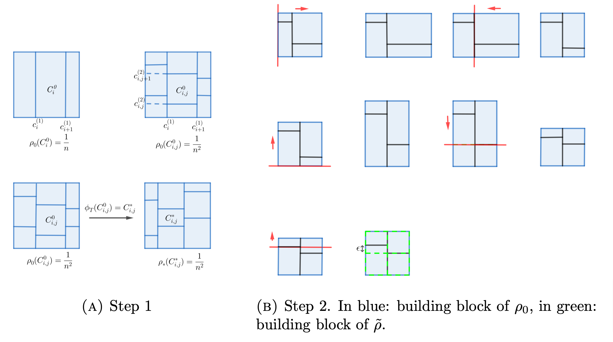
Figure 3. Qualitative representation of the proof of 2.
3. Conclusion
We have developed a constructive theory for the problems of interpolation, and partially for the problem of transport, with the general model (1.2). Our results show an interesting interplay between the number of neurons p and the number of discontinuities of the controls (i.e the number of layers). Indeed, by acting on the number of neurons p we can transition from the Tight NODEs (1.4) to an architecture closer to the Shallow NODEs (1.3). This is a first step towards a constructive theory of Shallow ResNets.
These results and observations illustrate how we can benefit from the theory of dynamical systems and control, to have a better understanding of neural networks, and uncover theoretical guarantees. This opens many interesting questions and avenues of research, which we plan to investigate in the near future.
References
[1] M. Benning, E. Celledoni, M. J. Ehrhardt, B. Owren, and C.-B. Sch¨onlieb. Deep learning as optimal control problems: models and numerical methods, 2019.[2] B. Chang, L. Meng, E. Haber, F. Tung, and D. Begert. Multi-level residual networks from dynamical systems view, 2018.
[3] R. T. Q. Chen, Y. Rubanova, J. Bettencourt, and D. Duvenaud. Neural ordinary differential equations, 2019.
[4] C. Cuchiero, M. Larsson, and J. Teichmann. Deep neural networks, generic universal interpolation, and controlled odes, 2020.
[5] G. Cybenko. Approximation by superpositions of a sigmoidal function. Mathematics of Control, Signals and Systems, 2(4):303–314, 1989.
[6] W. E, J. Han, and Q. Li. A mean-field optimal control formulation of deep learning. Research in the Mathematical Sciences, 6(1), 2018.
[7] Q. Li, L. Chen, C. Tai, and W. E. Maximum principle based algorithms for deep learning, 2018.
[8] Q. Li and S. Hao. An optimal control approach to deep learning and applications to discrete-weight neural networks, 2018.
[9] Q. Li, T. Lin, and Z. Shen. Deep learning via dynamical systems: An approximation perspective, 2020.
[10] Y. Lu, C. Ma, Y. Lu, J. Lu, and L. Ying. A mean-field analysis of deep resnet and beyond: Towards provable optimization via overparameterization from depth, 2020.
[11] Y. Lu, A. Zhong, Q. Li, and B. Dong. Beyond finite layer neural networks: Bridging deep architectures and numerical differential equations, 2020.
[12] P.-M. Nguyen and H. T. Pham. A rigorous framework for the mean field limit of multilayer neural networks, 2023.
[13] D. Ruiz-Balet, E. Affili, and E. Zuazua. Interpolation and approximation via momentum resnets and neural odes, 2021.
[14] D. Ruiz-Balet and E. Zuazua. Neural ode control for classification, approximation and transport, 2021.
[15] P. Tabuada and B. Gharesifard. Universal approximation power of deep residual neural networks through the lens of control. IEEE Transactions on Automatic Control, 68(5):2715–2728, 2023.
[16] C. Villani. Optimal transport: Old and new. Springer-Verlag Berlin, 2016.
[17] E. Weinan. A proposal on machine learning via dynamical systems. Communications in Mathematics and Statistics, 5(1):1–11.
|| Go to the Math & Research main page


