
Gas networks at stationary states: Analysis, software and visualization

Code: ![]()
Files to run: nocircle.m, onecircle.m or twocircles.m
1 Introduction
This post presents the results of my Bachelor thesis about the modeling and implementation of gas networks at stationary states. Using the isothermal Euler equations to describe the gas flow through a single pipe, algebraic node conditions that require the conservation of mass and the continuity of the pressure are needed to extend the model to general networks. A non-constant compressibility factor models the relationship between density and pressure occurring in real gas.
Additionally to the theoretical results that will be presented, I wrote a program to find a numeric solution that describes the stationary states on arbitrary finite networks. At the end, two examples will be dealt with by using the program to solve for the unique solution, of which existence is proven in the first part.
2 Derivation of the pressure function
In the following, the stationary state of the pipe flow will be described as in [4] by using the 1-d isothermal Euler equations. Since it can be observed that supply and demand remain constant for certain time intervals, it is useful to have a closer look at stationary state. An overview of different models for the description of gas flow in networks is given in [2].
First, we will derive a formula for the pressure drop within one pipe.
Let p denote the pressure and \alpha \in \left(-0.9,0\right). Then the compressibility factor z for real gas is given by
z(p) = 1 + \alpha p. (1)
In the case of ideal gas \alpha would be equal to 0 and thus z constant one. For a detailed description of stationary states in pipeline networks with ideal gas see [3].
Furthermore, the state equation for real gas
p = RTz(p) \rho (2)
will be used. R denotes the specific gas constant, T is the temperature and \rho the gas density. In this approach, T is constant within the whole network. In [1], coupling conditions for an intersection of pipes with variable temperatures are derived.
A relation between the sound speed c in the gas and the gas density \rho is given by
\left ( \frac{1}{c} \right )^2 = \frac{\partial\rho}{\partial{p}}. (3)
Let q be the mass flow rate, D the diameter of the pipe and \lambda_{fric}(x) > 0 the space-dependent Lipschitz continuous friction coefficient. Define \theta = \frac{\lambda_{fric}(x)}{\quad D}.
Finally, the central equations that govern the flow through a single horizontal pipe are given by the isothermal Euler equations
\color{black}\left\{ \begin{array}{l} \rule {0pt}{10pt}\rho_t + q_x = 0,\\ \rule {0pt}{15pt} q_t + \left(p + \frac{q^2}{\rho}\right)_x = -\frac{1}{2}\theta \frac{q\left|q\right|}{\rho}. \end{array} \right.
Consider the pipe as an interval of the length L > 0 with the boundary points x_0 = 0 and x_1= L.
Since only stationary states are considered, all time derivatives are equal to zero. Therefore, the first Euler equation implies that q is constant in x. Reformulating (2) and using q_t = 0 yields
\left( 1 - \left( \frac{q}{p}\right)^2 RT \right)p_x = -\frac{1}{2}\theta q \left| q\right | RT \left( \alpha + \frac{1}{p}\right). (4)
Define \eta = \left( \frac{v}{c} \right)^2 to be the square of the Mach number where the velocity v is given by
v = \frac{q}{\rho} = qRT \left( \alpha + \frac{1}{p}\right).
Inserting (2) in (3) leads to
\eta = \left(RT \left( \alpha + \frac{1}{p}\right) q \right)^2 \frac{\space 1}{RT}\frac{\quad 1}{\left( 1+\alpha p \right)^2} = RT \left( \frac{q}{p} \right)^2.
This result can be used to reformulate the factor in front of p_x in (4).
After multiplying (4) by \frac{ \quad p}{\alpha p +1} this differential equation can be solved by using separation of variables to get
\frac{p}{\alpha} + \left(q^2RT-\frac{1}{\alpha^2}\right)\ln(\left|1+\alpha p\right|) - q^2RT\ln(p) = C - \frac{1}{2}RT q \left| q \right|\int_{x_0}^x \theta (s) ds \text{,} \quad C \in \mathbb{R}. (5)
For p \in \left(0,\frac{\space 1}{\left|\alpha\right|}\right) define the left hand side of (5) as an auxiliary function F(p). It can be shown that for subsonic flow (\eta \lt 1) F(p) is strictly increasing, differentiable and strictly convex on \left( \left| q \right| \sqrt{RT}, \frac{\space 1} {\left| \alpha \right| }\right) and thus invertible on the same interval.
Summing everything up we get
\boxed{p(x,q,p_0) = F^{-1}\left( F(p_0) - \frac{1}{2}RT q \left| q \right|\int_{x_0}^x \theta (s) ds\right)} (6)
Remark
The inverse function F^{-1} can be evaluated by using Newton’s method. For a given z>F(\left|q\right|\sqrt{RT}) define
\phi(y) := F(y) - z.
Then it holds that
\phi(y) = 0 \Leftrightarrow F(y) = z \Leftrightarrow y = F^{-1}(z).
Since F is continuous an strictly increasing on \left(\left|q\right|\sqrt{RT},\frac{\space 1}{\left|\alpha\right|}\right), the same holds for \phi. Together with
\phi(\left|q\right|\sqrt{RT}) \lt 0 \text{ and } \lim_{y \nearrow} \frac{\space 1}{\left|\alpha\right|} F(y) = \infty
this shows the unique existence of a root y^* \in \left(\left|q\right|\sqrt{RT},\frac{\space 1}{\left|\alpha\right|}\right) such that y^* = F^{-1}(z).
Due to the convexity of F, the Newton iteration
y_{n+1} = y_n - \frac{\phi(y_n)}{\phi'(y_n)}, \quad y_0 \in \left( y^*,\frac{\space 1}{\left|\alpha\right|}\right) generates a monotonically decreasing sequence that converges to y^*.
3 Stationary states on networks
Having analysed the pressure drop in a single pipe, it is now possible to extend the model to an arbitrary network using coupling conditions. The first step is to describe the network, that can be seen as a graph G, by a matrix A.
Let therefore a finite connected directed graph G = (V,E) be given. Then, each edge e \in E corresponds to an interval [0,L^e]. Define E_0(v) = \left \{e\in E: e \text{ incident to } v \in V\right\} and let x^e(v) \in \left\{0,L^e\right\} be the end of the interval [0,L^e] that is adjacent to v. Define
\sigma(e,v) = \left\lbrace \begin{array}{ll} -1 \text{ if }x^e(v) = 0 \text{ and } e\in E_0(v)\\ 1 \text{ if } x^e(v) = L \text{ and } e\in E_0(v)\\ 0 \text{ if } e \not\in E_0(v) \end{array} \right.
The incidence matrix A\in\mathbb{R}^{|V|\times|E|} describing G is then given by A_{ij} = \sigma(e_j,v_i).
In general one can see that \text{dim}(\text{ker}(A)) is equal to the number of circles in the graph and that the vectors describing linearly independent circles form a basis of ker(A).
For all e,f\in E_0(v) the continuity of the pressure is given by
p^e(x^e(v)) = p^f(x^f(v)) \quad \forall v \in V. (7)
For all inner nodes the Kirchhoff condition is given by
\sum_{e\in E_0(v)} \sigma(e,v) (D^e)^2q^e(x^e(v)) = 0. (8)
Define the vector of outflows in all nodes by b \in \mathbb{R}^{|V|} such that
b\in B := \left\{ b \in \mathbb{R}^{|V|}: \sum_{v\in V} b_v = 0 \right\}. (9)
By using the connection
m^e = \frac{\pi}{4}(D^e)^2q^e
equation (8) and (9) can be rewritten as
A m = b, \quad m\in\mathbb{R}^{|E|}. (10)
Assuming that (D^e)^2 = (D^f)^2 for all e,f\in E this simplifies to
A q = b, \quad q\in\mathbb{R}^{|E|}.
Together with formula (6) for the pressure on a single pipe and conditions (7) and (10) the flow on an arbitrary finite network is uniquely determined.
Theorem 3.1.
Let a finite connected directed graph G = (V,E) be given and represented by its incidence matrix A with A_{ij} = \sigma(e_j,v_i). Each edge e\in E corresponds to an interval [0,L^e]. Define the space of admissible outflows
B := \left\{ b\in\mathbb{R}^{|V|}:\sum_{v\in V}b_v = 0\right\}.
In one boundary node v_0, a pressure p_0 \in \left(|b_{v_0}|\sqrt{RT},\frac{1}{|\alpha|}\right) is given.
Then there is a constant C(p_0,G) > 0 such that for every b\in B with a norm satisfying
||b|| \lt C(p_0,G)
there exists a unique subsonic stationary state (p,q)\in\mathbb{R}^{|V|} that satisfies
Am = b
and for v\in V for all e = (u,v)\in E_+(v) := \left\{ e\in E: e \text{ incident to } v\in V, \sigma(e,v) = 1\right\}\subset E_0(v) it holds
p_v = p^e(x(v),q^e,p_u).
Sketch of the Proof
The proof uses induction over dim(ker(A)) to reduce a network with n+1 circles to a network with n circles and one more unknown flow value \lambda. Then it needs to be shown, that \lambda is unique. For more details see [4].
Summing everything up, we have the following conditions that guarantee a uniquely determined network flow:
\boxed{ \begin{array}{rrllc} Am &=& b& & \text{(Kirchhoff Condition)} \\ p^e(x^e(v)) &=& p^f(x^f(v)) & \forall e,f\in E_0(v) & \text{(Arc Coupling)}\\ p_e(L^e) &=& p(L^e,p_e(0),q^e) & \forall e\in E & \text{(Node Coupling)} \end{array} }
4 Modeling and Implementation
In this part, numerically calculated solutions will be presented. First of all, due to Theorem 3.1 it is known, that there exists a unique solution for the networks fulfilling the required conditions. However, it does not give an explicit solution, but nevertheless, important information that can be used in the implementation:
A function calculates the pressure difference in every node v \in V by taking every possible path to reach node v starting from v_0. Then the differences in every single node are squared and summed up to get a total pressure difference for the whole network. In the end, this function has to be 0, since we know from theory, that the pressure continuity is a necessary condition for the solution (p,q).
Example 4.1
The network shown in Figure 1 contains one circle and two outflow nodes and b = \left( -120,0,0,0,90,30\right)^{T}. Figure 2 shows the corresponding flow values q. As expected, q_5 is much larger than q_6, and as a consequence, the pressure in node v_5 is smaller than in v_6. To explain this output one can use the fact that \partial_q p(x,q,p_0) \lt 0 for q \neq 0.
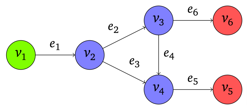
Figure 1. A network with one circle
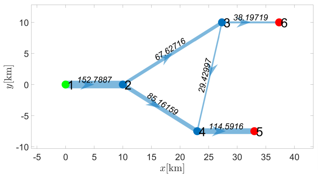
Figure 2. Output graph with flow values q at the edges (in kg s^{-1} m^{-2}).
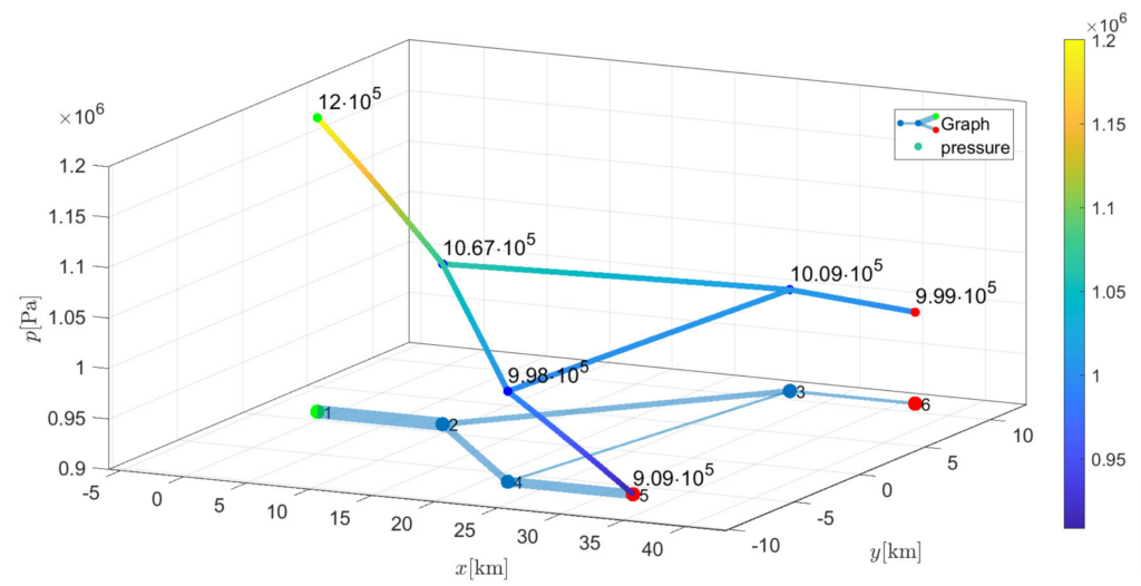
Figure 3. Pressure drop along a network with one circle
Example 4.2
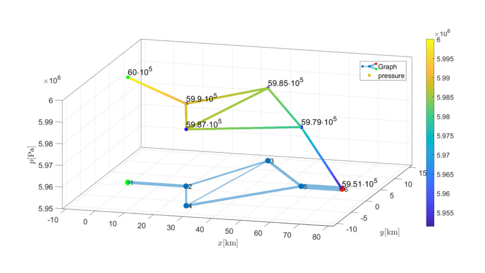
Finally, a diamond-shaped graph as seen in Figure 4 is solved. This means there are two circles. Even though this graph seems to be symmetric, the lengths L = 1000\cdot\left( 20,20,11.3,22,11,17,14\right)^{T} are chosen unsymmetrically. This results in the fact that there is a pressure difference in node v_3 and node v_4 as seen in Figure 6.
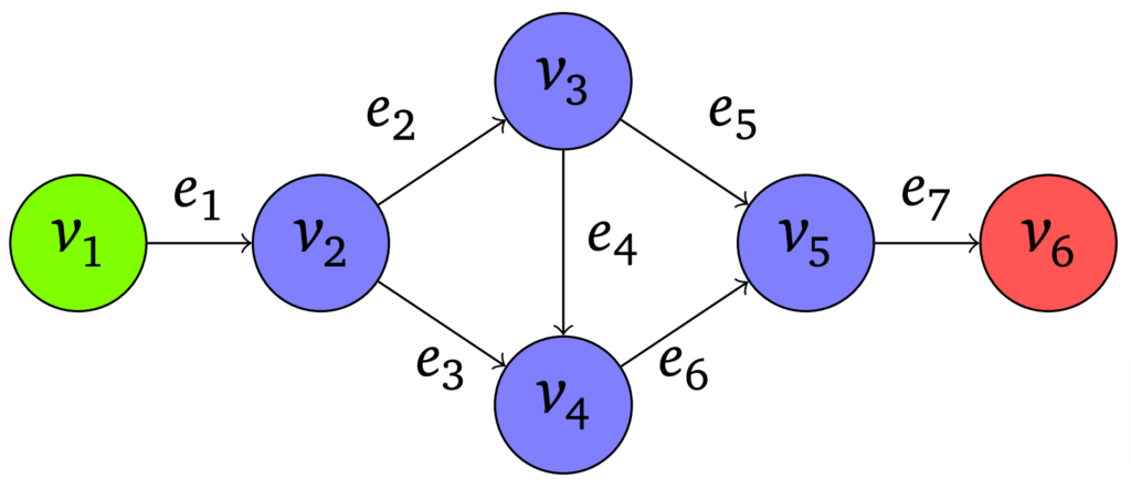
Figure 4. A diamond-shaped graph
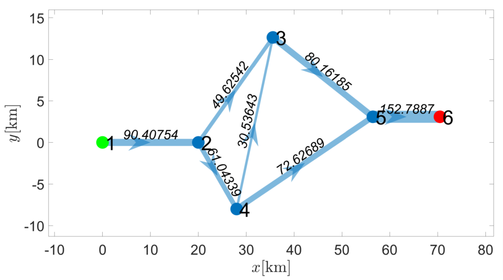
Figure 5. Output graph with flow values q at the edges (in kg s^{-1} m^{-2}).
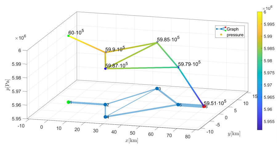
Figure 6. Pressure drop along a network with two circles
5 Outlook
Instead of looking at stationary states, one could also consider the time derivative not to be zero. The isothermal Euler equations then define a set of PDEs instead of ODEs. This means the approach to solve an initial value problem cannot be used anymore and must be extended to boundary value problems.
Since those boundary values representing the demands are usually uncertain, an ap- proach for optimization on gas networks under stochastic boundary conditions has been developed. The results are given in [6].
What is more, the approach presented in this post uses a compressibility factor z(p) = 1+\alpha p that is linearly dependent on p. This is not a necessary condition. The commonly used Weymouth equation for the pressure loss (see [5]) is given by
p^e_{weymouth}(x,q^e,p_0^e) = \sqrt{(p^e_0)^2-\theta^e x \left(c^e\right)^2 q^e |q^e|} (11)
where the sound speed is calculated via \left(c^e\right)^2 = RT^ez^e_m for a constant compressibility factor z^e_m.
Code: ![]()
Files to run: nocircle.m, onecircle.m or twocircles.m
References
[1] BANDA, Mapundi K. ; HERTY, Michael ; KLAR, Axel: Coupling conditions for gas networks governed by the isothermal Euler equations. In: Networks & Heteroge- neous Media 1 (2006), Nr. 2, S. 295[2] DOMSCHKE, Pia ; HILLER, Benjamin ; MEHRMANN, Volker ; MORANDIN, Riccardo ; TISCHENDORF, Caren: Gas network modeling: An overview. (2021)
[3] GUGAT, Martin ; LEUGERING, Günter ; HANTE, Falk: Stationary states in gas networks. In: Networks and Heterogeneous Media 10 (2016), Nr. 2, S. 295–320
[4] GUGAT, Martin ; SCHULTZ, Rüdiger ; WINTERGERST, David: Networks of pipelines for gas with nonconstant compressibility factor: stationary states. In: Computational and Applied Mathematics 37 (2018), Nr. 2, S. 1066–1097
[5] SCHROEDER, Donald W.: A tutorial on pipe flow equations. In: PSIG Annual Meeting OnePetro, 2010
[6] WINTERGERST, David: Optimization on Gas Networks under Stochastic Bound- ary Conditions, Friedrich-Alexander-Universität Erlangen-Nürnberg, dissertation, 2019
|| Go to the Math & Research main page


