

Null controllability for population dynamics with age, size structuring and diffusion

1. Motivation and description of age, size structured model
1.1. Motivation
Knowing the mechanisms of tumor growth can be useful for developing treatments. To mathematically describe its evolution from a global point of view, we can use a so-called “diffusion” equation. Diffusion equations are good tools in such a context, as they allow to describe the global effects of a physical process that takes place on a much smaller scale.
In this post, we are interested of the null controllability of population dynamics with age, size structuring and diffusion.
1.2. An example of an experimental device for the treatment of cancer
1.3. Description of age and size structured model
We consider the following system
\left\lbrace \begin{array}{ll} \dfrac{\partial y}{\partial t}+\dfrac{\partial y}{\partial a}+\dfrac{\partial (g(s)y) }{\partial s}-\Delta y+\mu(a,s)y=0 &\hbox{ in }\Omega\times (0,A)\times (0,S)\times(0,+\infty) ,\\ \dfrac{\partial y}{\partial \nu}=0&\hbox{ }(x,a,s,t)\in\partial\Omega\times(0,A)\times (0,S)\times(0,\infty),\\ y\left(x,0,s,t\right) =y^{1}_{i}(x,s,t)&\hbox{ } (x,s,t)\in\Omega\times (0,S)\times(0,\infty) \\ y\left(x,a,s,0\right)=y_{0}\left(x,a,s\right)& \hbox{ }(x,a,s)\in \Omega\times(0,A)\times (0,S);\\ y(x,a,0,t)=0& \hbox{ } (x,a,t)\in\Omega\times(0,A)\times(0,\infty). \end{array} \right. (1.1)
where y(x,a,s,t) (carcinogenic cells) is a distribution of individuals of age a size s at time t and location x\in\Omega. A and S are respectively the maximal live expectancy and the maximal size, \mu(a,s) natural death rate of individuals of individual.
1. \dfrac{\partial y}{\partial a} is the aging
2. \dfrac{\partial (g(s)y) }{\partial s} is the growing
3. \mu(a,s)y is the damping
4. y^{1}_{i}(x,s,t) \hbox{, }i\in\{1,2\} is the birth the rate, here we consider two type of birth rate.
(a) y^{1}_{1}(x,s,t)=\displaystyle\int\limits_{0}^{A}\int\limits_{0}^{S}\beta_1(a,\hat{s},s)y(x,a,\hat{s},t)da d\hat{s}.
Here \beta_1 is a positive function describing the fertility rate age-size, which depends on (a,\hat{s}) and also depending on the size s of the newborns.
In probabilistic terms, fertility \beta_1 can mean the probability of an individual of age a and of size \hat{s} giving birth to an individual of size s.
and
(b)
y^{1}_{2}(x,s,t)=\displaystyle\int\limits_{0}^{A}\beta_2(a,s)y(x,a,s,t)da
(c) It is assumed that size increases in the same way for everyone in the population and is controlled by the growth function g(s), then \dfrac{\partial (g(s)y) }{\partial s} is the growth. Here g(s)=1.

Figure 1. A Brain Implant Stops Tumor Growth in Rats
1.4. Existence and uniqueness result
Proposition 1.1. Description of age and size structured model. According to Gleen Webb, if the mortality and fertility rates \mu(a,s)=\mu_1(a)+\mu_2(s) and \beta_i are such that:
(H1): \left\lbrace \begin{array}{l} \mu_1(a)\geq 0 \text{ for every } a\in (0,A)\\ \mu_1\in L^{1}\left([0,a^*]\right)\hbox{ for every }\; a^*\in [0,A) \\ \displaystyle\int\limits_{0}^{A}\mu_1(a)da=+\infty \end{array} \right.,\quad
(H2): \left\lbrace\begin{array}{l} \mu_2(s)\geq 0 \hbox{ for every } s\in (0,S)\\ \mu_2\in L^{1}\left([0,s^*]\right)\hbox{ for every }\hbox{ } s^*\in [0,A) \\ \displaystyle\int\limits_{0}^{S}\mu_2(s)ds=+\infty \end{array} \right.
(H3): \left\lbrace\begin{array}{l} \beta_i\in L^{\infty}\hbox{, }i\in\{1,2\}\cr \beta_i \ge 0 \quad {\rm \; a.e.} \quad i\in \{1,2\},\\ \end{array} \right.
for any initial condition y_0\in K=L^2\left(\Omega\times (0,A)\times (0,S)\right), the system (1) admits a unique solution.
2. Observation and null controllability
2.1. The Null controllability problem
We consider the following system
\left\lbrace\begin{array}{ll} \dfrac{\partial y}{\partial t}+\dfrac{\partial y}{\partial a}+\dfrac{\partial y }{\partial s}-\Delta y+\mu(a,s)y=u\chi_{\Theta} &\hbox{ in }\Omega\times (0,A)\times (0,S)\times(0,\infty) ,\\ \dfrac{\partial y}{\partial \nu}=0&\hbox{ }(x,a,s,t)\in\partial\Omega\times(0,A)\times (0,S)\times(0,\infty),\\ y\left(x,0,s,t\right) =y^{1}_{i}(x,s,t)&\hbox{ } (x,s,t)\in\Omega\times (0,S)\times(0,\infty)\hbox{, }i\in\{1,2\} \\ y\left(x,a,s,0\right)=y_{0}\left(x,a,s\right)& \hbox{ }(x,a,s)\in \Omega\times(0,A)\times (0,S);\\ y(x,a,0,t)=0& \hbox{ } (x,a,t)\in\Omega\times(0,A)\times(0,\infty). \end{array}\right. (2.1)
where
1. \Theta=\omega\times(a_1,a_2)\times (s_1,s_2);
2. u(x,a,s,t) is the control;
3. \omega\times(a_1,a_2)\times (s_1,s_2)\subset \Omega\times (0,A)\times (0,S) is the support of the control;
4. Goal: To drive the solution to equilibrium at a given final time T>0
y(.,.,.,T)\equiv 0
2.2. The dual observation
Since the controllability of the linear system is equivalent to an observability inequality, we consider the adjoint system:
\left\lbrace\begin{array}{ll} \dfrac{\partial q}{\partial t}-\dfrac{\partial q}{\partial a}-\dfrac{\partial q}{\partial s}-\Delta q+\mu(a,s)q=q_i(x,s,t)&\hbox{ in }\Omega\times(0,A)\times (0,S)\times(0,+\infty) i\in\{1,2\},\\ \dfrac{\partial q}{\partial \nu}=0&\hbox{ }(x,a,s,t)\in\partial\Omega\times(0,A)\times (0,S)\times(0,\infty),\\ q\left( x,A,s,t\right) =0&\hbox{ in } (x,s,t)\in\Omega\times (0,S)\times(0,\infty) \\ q(x,a,S,t)=0& \hbox{ in } (x,a,t)\in\Omega\times(0,A)\times (0,\infty)\\ q\left(x,a,s,0\right)=q_0(x,a,s)& \hbox{ in }(x,a,s)\in\partial\Omega\times(0,A)\times (0,S); \end{array}\right. (2.2)
with the following correspondence
q_1(x,s,t)=\displaystyle\int\limits_{0}^{S}\beta_1(a,s,\hat{s})q(x,0,\hat{s},t)d\hat{s}\hbox{ matches with }y^{1}_{1},
and
q_2(x,s,t)=\beta_2(a,s)q(x,0,s,t)\hbox{ matches with }y^{1}_{2}.
2.3. The dual observation problem
The null controllability problem therefore becomes an observability inequality problem and the question is whether:
is the inequality
\displaystyle\int\limits_{0}^{S}\int\limits_{0}^{A}\int_{\Omega}q^2(a,s,T)dxdads\leq K_T\displaystyle\int\limits_{0}^{T}\int\limits_{s_1}^{s_2}\int\limits_{a_1}^{a_2}\int_{\omega}q^2(a,s,t)dadsdt.
verified?
The observation being made in the subset
\omega\times(a_1,a_2)\times (s_1,s_2)\subset \Omega\times (0,A)\times (0,S).
2.4. Null controllability results
The answer to the previous question is affirmative and we have the following null controllability result.
We denote by T_1=\max\{a_1+S-s_2,s_1\}\hbox{ and }T_0=\max\{S-s_2,s_1\}.
Theorem 2.1
The null controllability result holds in \omega\times(a_1,a_2)\times (s_1,s_2)\subset \Omega\times (0,A)\times (0,S) with
T_0 \lt \min\{a_2-a_1,\hat{a}-a_1\}; provided the fertility rate is such that \beta_i(a,.)\equiv 0\hbox{ in }(0,a_1+\gamma), and the time T is large enough such that:
1. for the birth rate equal y^{1}_{1}, T>A-a_2+T_1+T_0 and
2. for the birth rate equal y^{1}_{2}, T>A-a_2+a_1+S-s_2+s_1.
2.5. Idea of Proof
2.5.1. Change of variables
The proof of the observability inequality is based on the estimation of the non-local term q_i\hbox{, }i\in\{1,2\}.\\
As \beta(a,.)\equiv 0\hbox{ in }(0,a_1+\gamma), the first equation of the adjoint system become
\dfrac{\partial q}{\partial t}-\dfrac{\partial q}{\partial a}-\dfrac{\partial q}{\partial s}-\Delta q+\mu(a,s)q=0\hbox{ in }\Omega\times(0,\hat{a})\times (0,S)\times(0,+\infty).
We denote by \tilde{q}(x,a,s,t)=q(x,a,s,t)\exp\left(-\int\limits_{0}^{a}\mu_1(\alpha)d\alpha-\int\limits_{0}^{s}\mu_2(r)dr\right).w(x,\lambda)=\tilde{q}(x,t-\lambda,s+t-\lambda,\lambda) \text{ ; }x\in\Omega\hbox{, }\lambda\in (0,t).
2.5.2. Estimation of the non local term
Then w satisfies:
• \dfrac{\partial w(x,\lambda)}{\partial \lambda}-\Delta w(x,\lambda)=0\text{ in } \Omega\times (0,t).
• The q(x,0,s,t) can be estimate from the observation; according to the variables s and t. Indeed, for s\in (0, S_2-a_1), we can estimate q(x,0,s,t) from the observation for all t \gt \max\{a_1,s_1\} and for s\in (S_2-a_1,S), we can estimate q(x,0,s,t) from the observation for all t \gt a_1+S-s_2.
• Then the sum q_{1} can be estimate for all time t \gt T_1.
3. Illustration of the observability inequality
3.1. Illustration of the estimate of q(x,0,s,t)
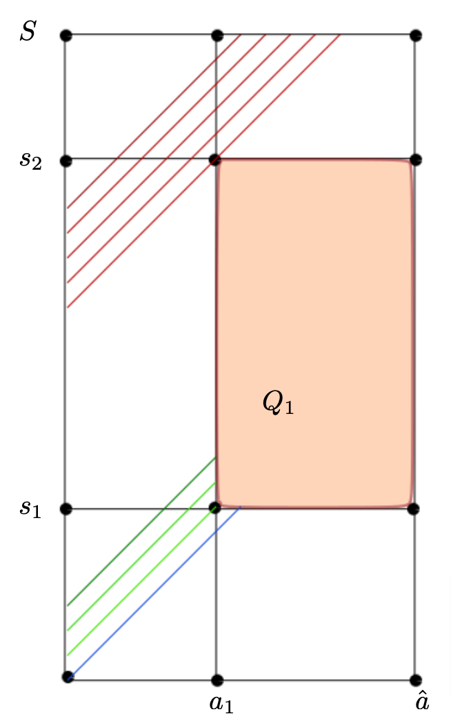
Figure 2. Here T_0 \lt \min\{a_2-a_1,\hat{a}-a_1\} and we choose a_2=\hat{a}. Since t \gt T_1 all the backward characteristics starting from (0,s,t) enters the observation domain (the green and blue lines), or without the domain by the boundary s=S (red line).
3.2. Illustration of cases where we are not able to estimate q(x,0,s,t)
3.2.1. Graphical proof of the condition T_0=S-s_2 \lt \min\{a_2-a_1,\hat{a}-a_1\}
FIGURE_3
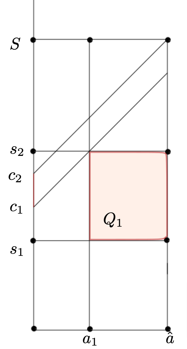
Figure 3. For S-s_2 \gt \hat{a}-a_1, we can not estimate q (x,0,s,t) for s\in(c_1,c_2) by the characteristic method. Indeed for even t \gt a_1+S-s_2 the characteristics starting at (0,s,t) without the domain by the boundary t=0 \hbox{ or enter in the region } a \gt \hat{a}, without going through the observation domain.
3.3. Graphical proof of the condition T_0=s_1 \lt \min\{a_2-a_1,\hat{a}-a_1\}
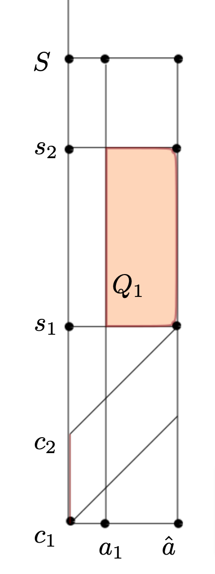
Figure 4. For the second case if s_1 \gt \hat{a}-a_1, we can not estimate q (x,0,s,t) for s\in (c_1,c_2) by the characteristic method. Indeed for even t>a_1+S-s_2 the characteristics starting at (0,s,t) without the domain by the boundary t=0 \hbox{ or enter in the region } a>\hat{a}, without going through the observation domain.
3.4. Minimal time
3.4.1. Graphical proof of minimal time
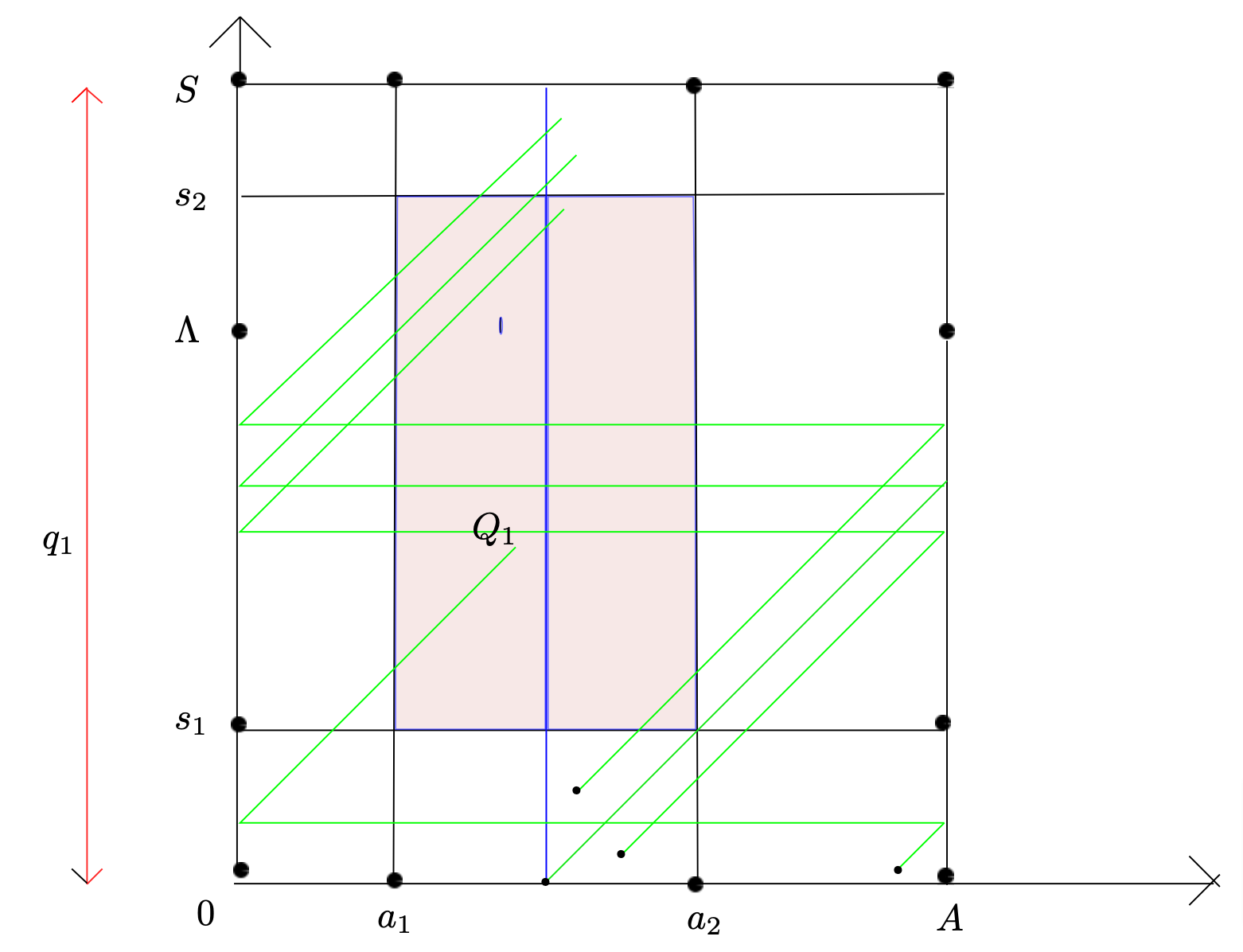
Figure 5. \Lambda=s_2-a_1. The backward characteristics starting from (a,s,T) with a\in (a_0,A) (red lines or green lines) hits the boundary (a=A), gets renewed by the renewal condition q_1 and then enters the observation domain (green lines) or without by the boundary s=S.
3.4.2. Graphical proof of minimal time
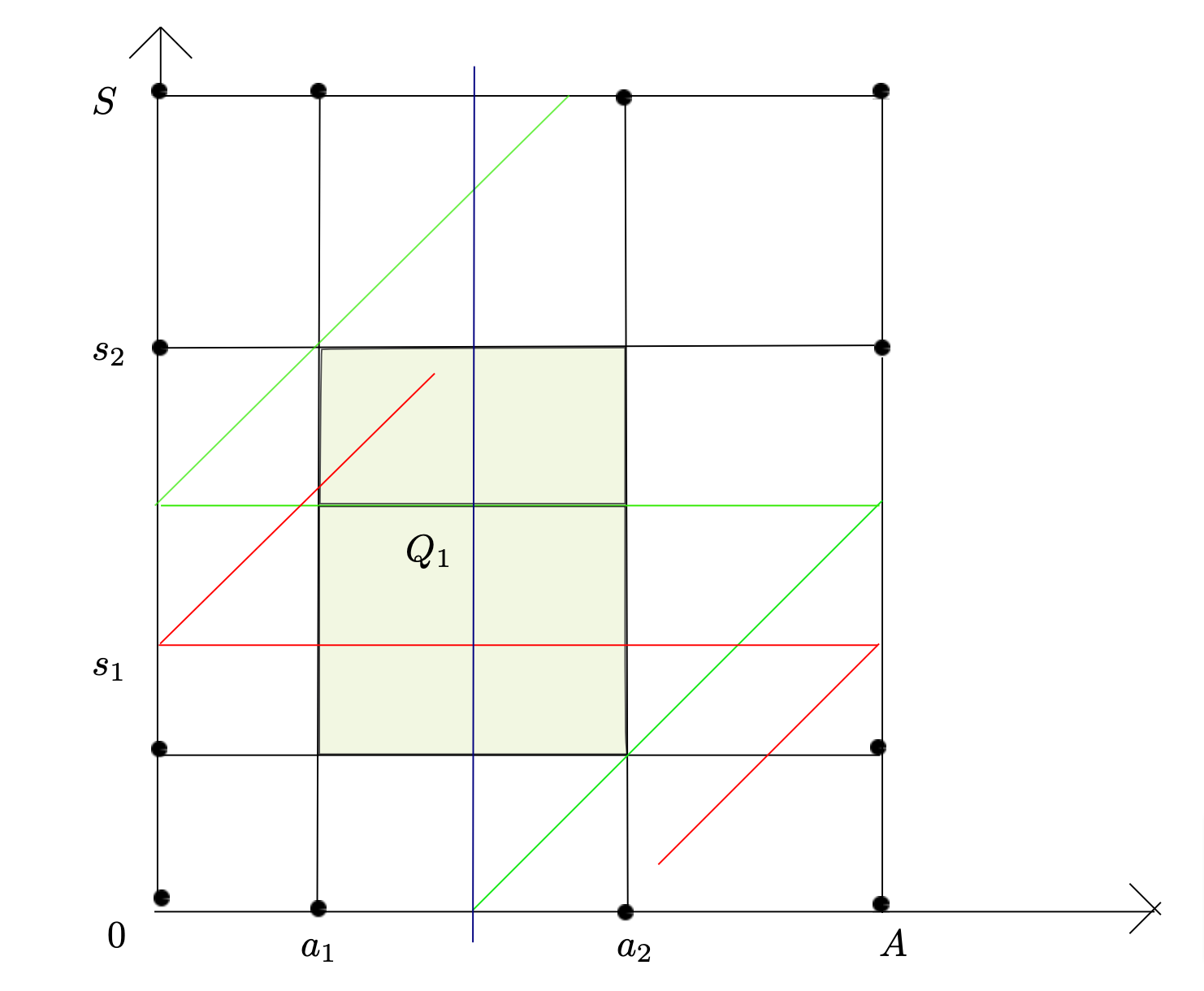
Figure 6. Here \hat{a}=a_2. The backward characteristics starting from (a,s,T) hits the boundary (a=A), gets renewed by the renewal condition q_2 and then enters the observation domain (red line) or without and leave the domain \Sigma by the boundary s=S (green line)
References
[1] Y. Simpore, U. Biccari. Controllability and Positivity Constraints in Population Dynamics with age, size Structuring and Diffusion (2022) arxiv: 10.48550/arXiv.2209.04018[2] Y. Simpore, Y. El gantouh, U. Biccari. Null Controllability for a Degenerate Structured Population Model (2022). arxiv: 10.48550/arXiv.2209.03645
|| Go to the Math & Research main page


