

Reinforcement Learning and LQR with special control structure: switched and multilevel systems
 Nicolas Schlosser
1 Introduction
In this post we study the well-known linear-quadratic regulator problem in continuous time
\dot{x}(t) = A x(t) + B u(t), \quad x(0) = x_0.
where t \in [0, T], A \in \mathbb{R}^{n \times n}, B \in \mathbb{R}^{n \times m}, x(t) \in \mathbb{R}^n, and x_0 is the initial state. The goal is to choose a control u: [0, T] \to \mathbb{R}^m in such a way that at time T, we have x(T) = \bar{x} for some target state \bar{x}. Often, for simplicity, we use \bar{x} = 0.
We also consider the time-discrete counterpart
x_{k+1} = A x_k + Bu_k, \quad x_{k = 0} = x_0
where x, A, B and x_0 are as before and k \in \{0, \ldots, K\}. This time, we have to find discrete control inputs u_0, \ldots, u_{K-1} such that we have x_K = \bar{x}, which again we often assume to be the zero vector.
These two problems have been known for a long time and are thus well studied. It turns out that the conditions for the existence of controls u such that the target condition is fulfilled are the same for both problems: the matrix
(B, AB, A^2 B, \ldots, A^{n-1} B)
must have full rank n. In the time-discrete setting, we additionally have to assume that K \geq n. The condition on the rank of the so-called controllability matrix is known as the Kalman rank condition. If it holds, a control u: [0, T] \to \mathbb{R}^m for the continuous-time problem with \bar{x} = 0 can be found by looking for minimizers p_T^* of the functional
J(p_T) = \frac 12 \int_0^T \vert B^\top p \vert^2 dt + \langle x_0, p(0) \rangle
under the condition
-\dot{p}(t) = A^\top p(t), \quad p(T) = p_T
(the so-called adjoint equation) and then letting u(t) = B^\top p^*(t).
However, there are more possibilities, and therefore we might wonder what happens when we prescribe additional structure constraints to the control u. Examples are:
• Suppose that m = 2. Can we then find a control where at every time, only one of the two components u_1(t), u_2(t) is active while the other one rests at zero? In other words, can we find u in such a way that
u_1(t) \cdot u_2(t) = 0
holds for almost every t \in [0, T]? A control u with this form is called a switching control. Generalizations for m \geq 2 are possible.
• The u found by the method above is continuous with respect to time. It might be preferable to look for other properties, for example that u only takes values from a finite set of admissible controls. More formally, if \mathcal{R} = \{\rho_1, \ldots, \rho_N\} where each \rho_n \in \mathbb{R}^m, we might ask if it is possible to find u: [0, T] \to \mathcal{R} such that x(T) = 0 holds. This type of control is called a multilevel, or when N = 2, a bang-bang control.
In the continuous-time setting, existence of switching, bang-bang, and multilevel controls has been established in multiple papers by Zuazua et. al., and the baseline idea for the proof is to modify the functional J given above. In discrete time, existence of a multilevel control cannot always be achieved, take for example m = n = 1, A = B = 1, then the goal is to find u_0, \ldots, u_{K-1} \in \mathcal{R} such that
u_0 + u_1 + \ldots + u_{K-1} = -x_0.
If for example K = 1 and -x_0 \notin \mathcal{R}, this is of course not possible. For general K, the control problem turns into the postage stamp problem, a famous problem in combinatorics. There are connections to number theory as well, e.g. Bézout’s lemma states that if \mathcal{R} = \{\pm\rho_1, \pm\rho_2\} \subset \mathbb{Z} and x_0 = 1, then for sufficiently large K there exist multilevel controls if and only if \rho_1 and \rho_2 are coprime.
We are interested in a different thing:
Can an agent that can freely interact with the system “learn” a control with the prescribed structure that drives the system to zero? Problems of this form can be solved using techniques from Reinforcement learning, which we introduce next.
2 Reinforcement Learning
The basic setting for Reinforcement Learning (which we are going to shorten to RL in what follows) is a set \mathcal{X} of states a system can be in, and another set \mathcal{A}(x) of actions an agent can perform in state x \in \mathcal{X} to change the state of the system. After an action a is chosen and the system transitions from x to a new state, a running cost g(x, a) is induced. Some states are so-called final states, where the system comes to a halt. If x is a final state, we induce a final cost g_f(x) and the current episode ends. The goal of the agent is to perform actions a_0, a_1, \ldots in such a way that once a final state x_f is reached, the total costs
g_f(x_f) + g(x_0, a_0) + g(x_1, a_1) + \ldots
are minimal. There are several methods (temporal difference learning, Q learning, first/every visit Monte Carlo, SARSA, …, to name a few) with different properties (model-based vs. model-free, off- vs. on-policy, value- vs. policy based, …) to tackle this problem, mostly by obtaining approximations for the so-called value function or, alternatively, for the action-value function of the system by interacting with it. We do not go into detail any further, the takeaway message is that once a problem has been cast into the RL framework, we can use existing methods to obtain solutions for it.
In the following, we explain how to formulate the special-structure LQR problem as RL problems, present our results, and comment about possible difficulties.
3 Warm-up: The classical problem
Formulating the classical LQR problem as a RL problem is easy and a great exercise to the interested reader; we add it here to have a comparison for later and to explain the methodology. We start with the time-discrete case. Let
\mathcal{X} = \{(x, k) \mid x \in \mathbb{R}^n, k \in \{0, \ldots, K\}\}
the set of possible states the system can be in. We have to include the time index k in the state space, otherwise we do not know when an episode should end. The action space \mathcal{A} does not depend on x and is simply given as
\mathcal{A} = \{u \mid u \in \mathbb{R}^m\}.
Choosing action u in state (x, k) yields the new state (Ax + Bu, k+1) with no running costs. Final states are those (x, k) where k = K, and the final cost is given by \|x - \bar{x}\|, where we can choose some norm on \mathbb{R}^n. Alternatives, such as \|x - \bar{x}\|^2, are also possible.
The continuous-time case already presents us the first problem: RL needs a discrete-time setting, since it has to choose a sequence of actions one after the other. The most common and intuitive approach is to choose a numerical scheme, e.g. the classical explicit Euler method, to approximate the dynamics. This works as follows: Given the stepsize \Delta t \coloneqq T/K, where we fix K \in \mathbb{N}, we approximate
x(t + \Delta t) \approx x (t) + \Delta t (A x(t) + B u(t)).
By letting x_k \coloneqq x(k \Delta t), we are back into the time-discrete case.
4 Switching controls
As we have seen in the previous section, the continuous-time setting is best handled by discretizing time. Hence, we only discuss the time-discrete case here. For simplicity, let m = 2 for the remainder of this section.
In order to include structure for a switching control, the framework we established for the classical problem is not sufficient, since we do not impose the switching condition at any point. Restricting \mathcal{A} to
\{u \in \mathbb{R}^2 \mid u_1 \cdot u_2 = 0\}
would yield switching controls, but gives no control over the switching process whatsoever. This might be impractical if we wish to minimize the number the control switches. However, we can achieve this by including the currently active control into the state space. So let
\mathcal{X} = \{(x, k, a) \mid x \in \mathbb{R}^n, k \in \{1, \ldots, K\}, a \in \{1, 2\}\}.
A triple (x, k, a) indicates that we have reached state x_k, and the previous control u_{k-1} satisfied (u_{k-1})_a \neq 0, (u_{k-1})_{3-a} = 0. (If k = 0, this is of course meaningless.) As action space, we separate the control value from the index where it is active:
\mathcal{A} \coloneqq \{(u, b) \mid u \in \mathbb{R}, b \in \{1, 2\}\}.
Now the transition is given as follows: Choosing action (u, b) in state (x, k, a) leads to the new state
(A x + B e_b u, k+1, b),
where e_1 = (1, 0) and e_2 = (0, 1) are the standard basis vectors. Now, in order to minimize the number of times where the control switches, we impose a running cost r if a \neq b and no costs if a = b. The final states and costs are as described in the previous section, with obvious adaptations. Fine-tuning the parameter r (to small will show no effect, too large will not drive the system to zero) allows us to control the number of switches.
If we want to implement this method on a computer, we also have to discretize the x and u variables. The discretization of u is easy, we can just take
\{-\bar{u}, -\bar{u} + \Delta u, -\bar{u} + 2 \Delta u, \ldots, \bar{u}\}
for some control bound \bar{u} and discretization parameter \Delta u. Discretizing x is harder, we cannot simply prescribe some set, as we have to make sure that a transition again yields a state from the set. However, it turns out that the RL algorithms do only need approximations for functions \mathcal{X} \times \mathcal{A} \to \mathbb{R}. By partitioning \mathbb{R}^n into sets \Omega_1, \ldots, \Omega_N, we can approximate functions on \mathbb{R}^n by step functions, which yields acceptable results. This process is known as state aggregation.
As an example, we consider the system
\dot{x}(t) = \begin{pmatrix} 1 & 0 \\ 0 & 2 \end{pmatrix} x(t) + \begin{pmatrix} 1 \\ 0 \end{pmatrix} u_1(x) + \begin{pmatrix} 0 \\ 1 \end{pmatrix} u_2(x)
and try to find controls u in such a way that the state of the system changes from x_0 = (2, -3)^\top at time 0 to \bar{x} = (-4, 7)^\top at time 1. In order to lower computational cost, our algorithm uses a coarse time grid with only five time steps, and a discretized control set \{-20, -15, -10, -5, 0, 5, 10, 15, 20\}. We compute ten million steps, which took over five hours to run, and evaluate every 10.000 iterations to check convergence. The results are displayed in Figure \ref{fig:switching}. We observe that despite the coarse discretization, the algorithm does a good job in finding a control that drives the system into the desired state.
The code used to generate these images is available at FAU DCN-AvH’s github: https://github.com/DCN-FAU-AvH/RL-Switching-Multilevel.
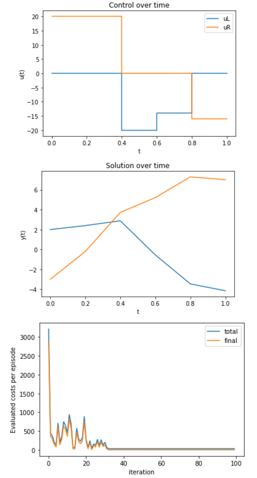
Figure 1. Learned results for a switching control system.
5 Multilevel control in discrete time
As we have mentioned above, the time-discrete multilevel control problem might nit always have a solution. However, the RL agent does not care about this, it simply chooses the controls in such a way that the overall costs are minimized, therefore finding some sort of approximate control, which might not be exactly the zero vector, but as close to it as it can get.
For simplicity assume that m = 1, i.e. all controls are scalars. A desirable property for controls is the so-called staircase property, i.e. for any k, the set (\min\{u_k, u_{k+1}\}, \max\{u_k, u_{k+1}\}) \cap \mathcal{R} should be empty. (Recall that \mathcal{R} = \{\rho_1, \ldots, \rho_N\} is the set of admissible controls. For later use we will assume that \rho_1 \lt \ldots \lt \rho_N.) In other words, the control can only switch to the next higher or next lower permitted value, not skipping any. It is easy for a RL agent to only look for controls with the staircase property. In addition, as with the switching controls, we might want to minimize the number of times where the control switches from one value to the next. Hence, we use a similar approach as for switching controls. We start with
\mathcal{X} = \{(x, k, \rho) \mid x \in \mathbb{R}^n, k \in \{1, \ldots, K\}, \rho \in \mathcal{R}\}.
Similar to before, a triple (x, k, \rho) represents that we have reached state x_k at time k from some other state by means of the control \rho. In order to enforce a staircase control, the action space must now depend on the state variable, but is otherwise just as in the classical setting:
\mathcal{A}(x, k, \rho_\ell) = \{\rho_{\ell-1}, \rho_\ell, \rho_{\ell+1}\}
(if \ell = 0 or \ell = N, then \ell \pm 1 is undefined and the respective element is missing from the set). Selecting the action u transfers the state (x, k, \rho) to the new state (Ax + Bu, k+1, u), and, if we wish, incurs a nonnegative switching cost if u \neq \rho. Final states and costs are defined just as in the previous sections, and similar state aggregation techniques can be used here.
As an example, we consider the system
x_{k+1} = \begin{pmatrix} -1 & 2\\ 0 & 1 \end{pmatrix} x_k + \begin{pmatrix} 0\\1 \end{pmatrix} u_k, \quad x_0 = \begin{pmatrix} 3\\1 \end{pmatrix}
and we want that x_{10} = \bar{x} = (0, 0)^\top.
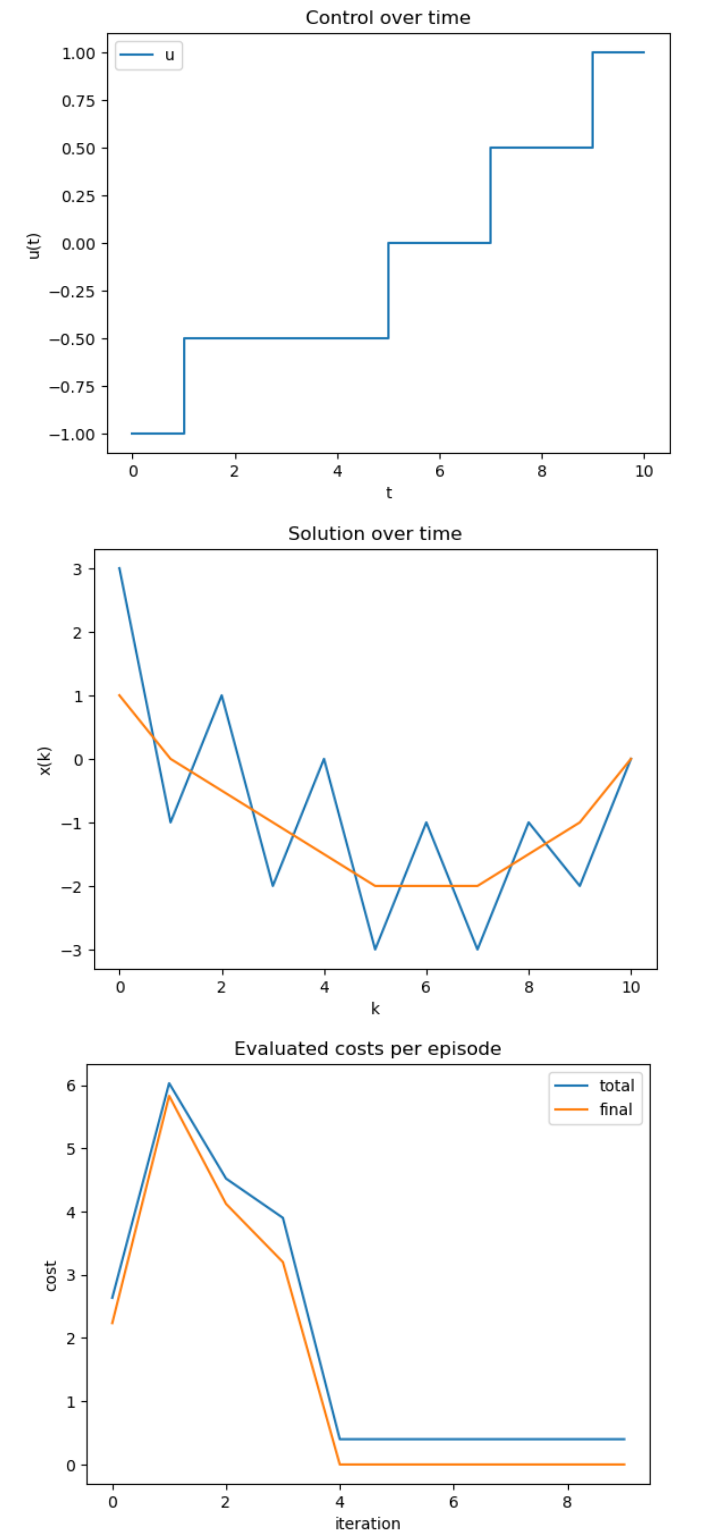
Figure 2. Learned results for a multilevel control system.
6 Outlook: Multilevel control in continuous time
If we want to solve the continuous-time multilevel control problem with RL techniques, we could start as before and discretize time using an explicit Euler scheme. However, as we have seen before, this might turn a solvable problem into an unsolvable one, which is of course not acceptable. A better way is, therefore, to not only learn which control to choose next, but also for how long, bypassing the need for time discretization. Another advantage of this approach is that we can easily include a nonnegative dwell time \delta, which represents the minimal time between switches. Our formulation is as follows: We start with
\mathcal{X} = \{(x, t, \rho) \mid x \in \mathbb{R}^n, t \in [0, T], \rho \in \mathcal{R}\},
similar to the time-discrete case. However, the action space changes, as we include the duration during which a control is active:
\mathcal{A}(x, t, \rho_\ell) = \{(u, \tau) \mid u \in \{\rho_{\ell-1}, \rho_{\ell+1}\}, \tau \in [\delta, T]\}.
The transition from a state (x, t, \rho) by choosing action (u, \tau) is given as follows: First, we calculate \tilde{t} \coloneqq \min\{t + \tau, T\}. In the next step, we look at the IVP
\dot{y}(s) = A y(s) + Bu, \quad y(t) = x
and define the next state by (y(\tilde{t}), \tilde{t}, u). We can also calculate y(\tilde{t}) directly as
y(\tilde{t}) = \exp((\tilde{t} - t) A) x + \int_t^{\tilde{t}} \exp((\tilde{t} - r) A) B dr \cdot u,
or alternatively use a numerical ODE solver, preferable without a fixed step size. Since we switch the control in every transition, the transition costs are just given by a constant value independent on the current state and action. Final states are those where t = T (this can even be checked on a machine without floating-point errors), and final costs are calculated as before.
The main differences to the procedure descried in the previous section are:
• The episodes do not have a fixed length. Having \delta > 0 ensures that episodes will end eventually after at most \lceil T/\delta\rceil transitions, but most of the time will take much less steps.
• We now have a continuous variable in the action space, namely \tau, which causes problems in actual implementations. This is because, in trying to find the optimal control strategy, RL algorithms minimize with respect to \tau, and if we approximate with step functions, the minimum is not unique, hence the optimal strategy remains unknown. More advanced function approximation has to be used, which usually comes at the price of higher computational needs. This problem is left for further research.
|| Go to the Math & Research main page


