Reinforcement learning as a new perspective into controlling physical systems

By Theïlo Terrisse, Visiting PhD Student. L’Ecole des Ponts ParisTech (France)

Introduction

Optimal control addresses the problem of bringing a system from an initial state to a target state, like a satellite that we want to send into orbit using the least possible amount of fuel. Since the last century, mathematics has helped develop powerful numerical methods for control. Many of these methods assume the system being controlled has linear dynamics. Unfortunately, this assumption often does not hold in real life. There are further reason why traditional control methods may fail:
1. They require an explicit mathematical model for the system being controlled.
2. They can require expensive computations that cannot be performed in real-time.
3. They suffer from the famous curse of dimensionality.

In this post, we explore how these problems can be tackled via reinforcement learning.

GitHub Repository

Download resources from our FAU DCN-AvH GitHub, at: https://github.com/DCN-FAU-AvH/RL-cart/tree/main

This repo contains the implementation of reinforcement learning (RL) algorithms for two linear-quadratic optimal control problems. Both consist in pushing a cart along a 1D-axis from a random initial position to a fixed target position; but each one illustrates different aspects of RL:

• The Sped-up-cart folder involves a reduced version of the problem for visualization purposes. It implements the Q-learning algorithm and visualizes the Q array for various parameters of the algorithm. It illustrates the exploration-exploitation dilemma in RL.
• The Accelerated-cart folder solves the full-fledged problem by training pre-implemented RL algorithms from the stable-baselines3 library. The problem is also solved using an adjoint method and the two approaches are compared.
Each of the two projects consists of source code and a notebook which defines and calls the main functions and gives comments on the results. The params.py file of each folder also defines the default parameters for the problem and the algorithms.

Requirements

To run the code, it is advised to create a new virtual Python environment and to install Jupyter.

Then, the required libraries are listed in the requirements.txt file of each project folder. To install them, simply enter the corresponding folder and run
pip install -r requirements.txt

What is reinforcement learning?

Reinforcement learning (RL) aims at using past experience of a system to decide how to match situations to actions so as to collect rewards over the system’s evolution.
The essence of RL is summarized in Figure 1. An agent evolves in an environment, observes its current state $s_t$ , and takes an action $a_t$ based on this observation. This action earns the agent a reward $r_t$ , which is large if the action moved the agent towards its goal, and low otherwise. The environment then comes into a new state $s_{t+1}$ and the process is repeated until some (finite or infinite) time-horizon $T$ .
The aim of RL is thus to design an agent so as to maximize the cumulative reward over time $\sum_{t=0}^{T-1} r_t$ ; that is not only the current reward but also future ones.

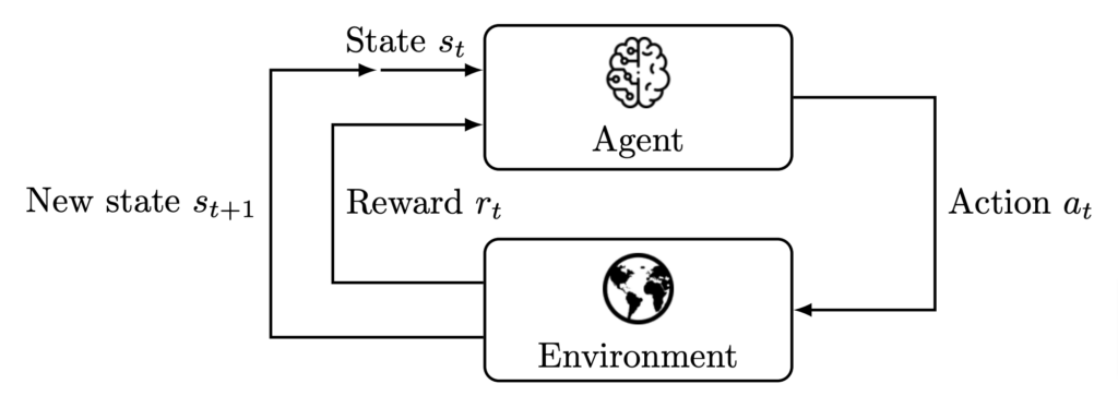
Figure 1. The agent–environment interaction in reinforcement learning, adapted from [3, Fig. 3.1].

Example: a mouse in a maze

Let’s illustrate RL on a very simple example. As in figure 2, suppose a mouse (the agent) is evolving in a maze (the environment) where cheese is hidden. The mouse moves inside the maze (the actions) so as to find the cheese as quickly as possible while avoiding a trap. The mouse earns a reward of -1 if it moves from one cell to another without finding cheese, a reward of +10 when it finds the cheese, and a reward of -10 when it falls in the trap. This mouse is very short-sighted but with a good memory: it can only see its current cell, but can recognize every cell it has visited.

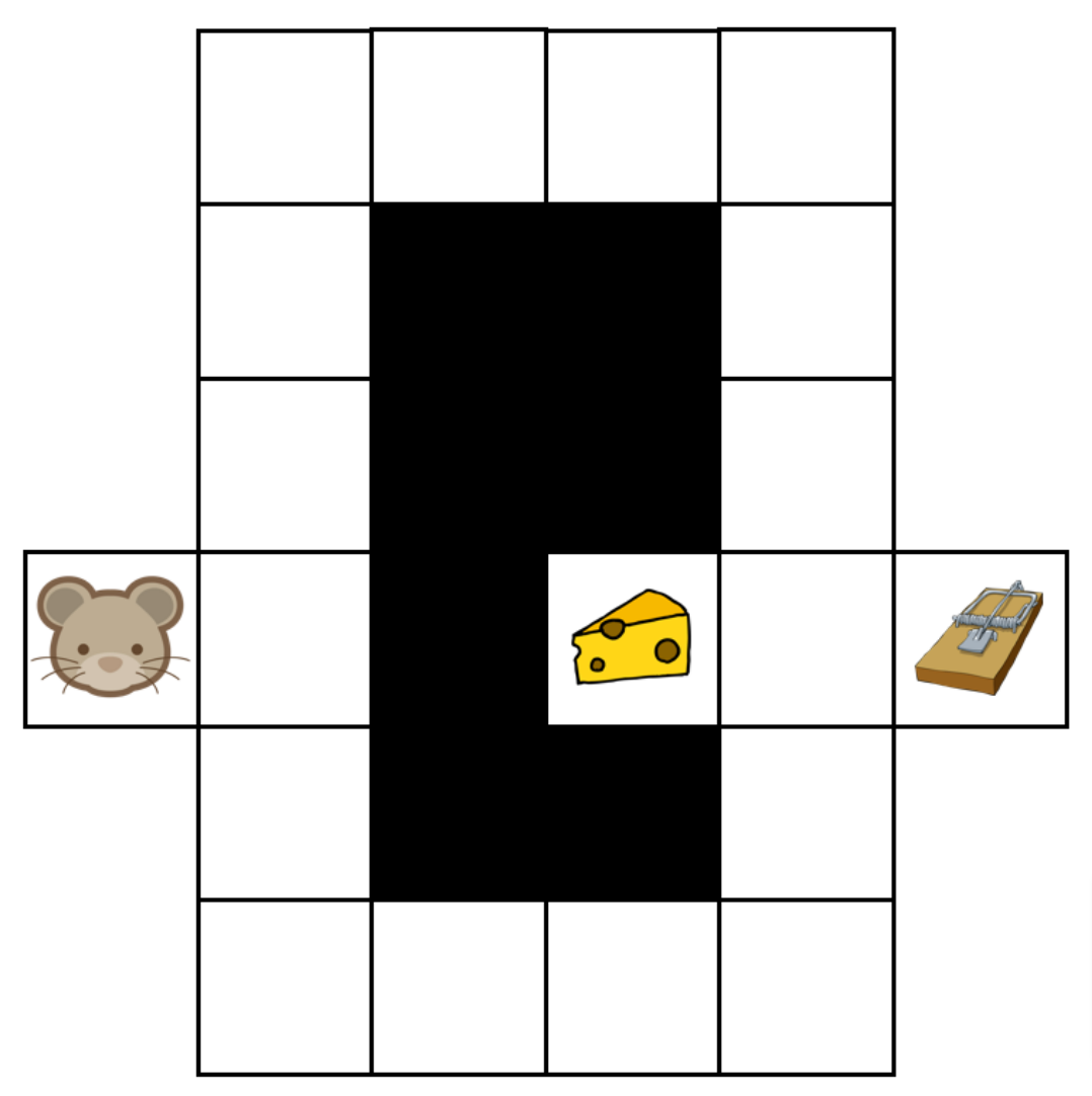
The maze example.

Initially, the mouse doesn’t know the maze and adopts an arbitrary behaviour according to the following preferences:
1. it prefers turning left over turning right;

2. it prefers turning right over going forward;

3. it prefers going forward over going backward.

An episode of the maze exploration process starts with the mouse on the left and ends when the mouse gets the cheese or the trap.

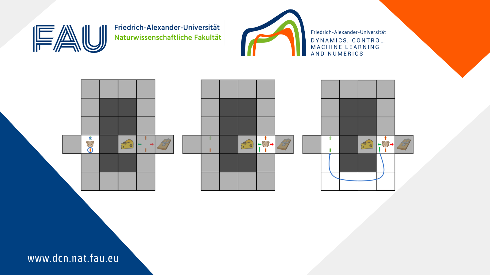
A first run through the maze gives the moves illustrated in Figure 3. In the figure, coloured arrows represent the mouse’s willingness to follow each direction (with increasing preference from red to green), and an action is taken by choosing the preferred direction.

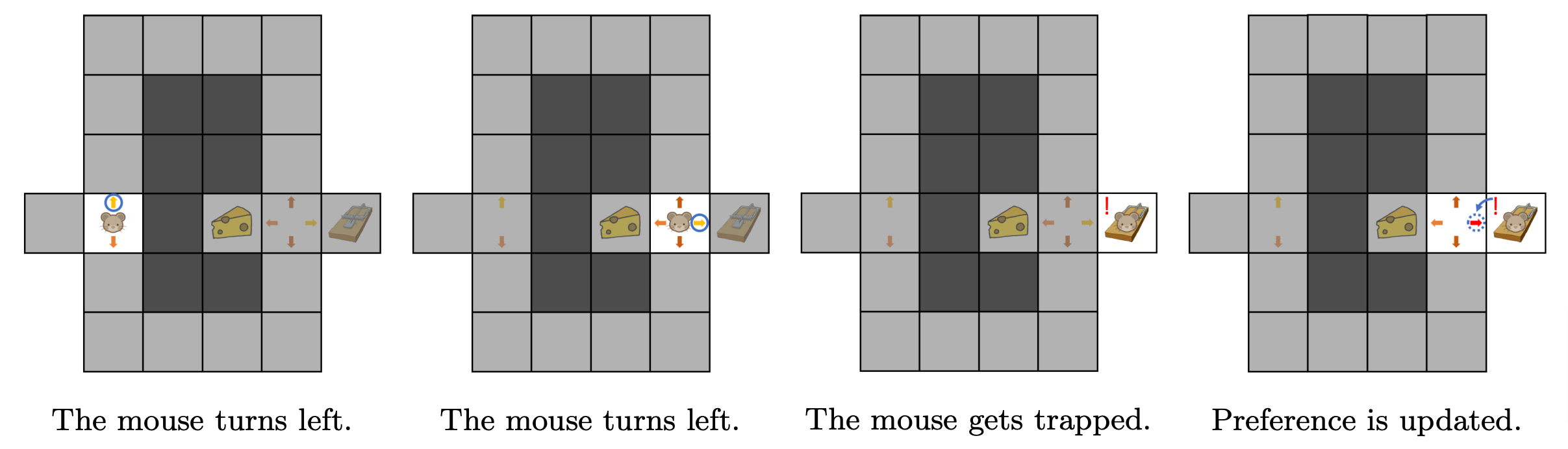Figure 3. First episode.

In this first episode, the mouse evaluated its initial behaviour by testing it. When it tries to solve the maze for the second time, the mouse will improve its behaviour using what it learned during the first run: taking a second turn left is not a good move because it leads to a trap. Thus, the second episode of maze exploration results in the behaviour shown in Figure 4.

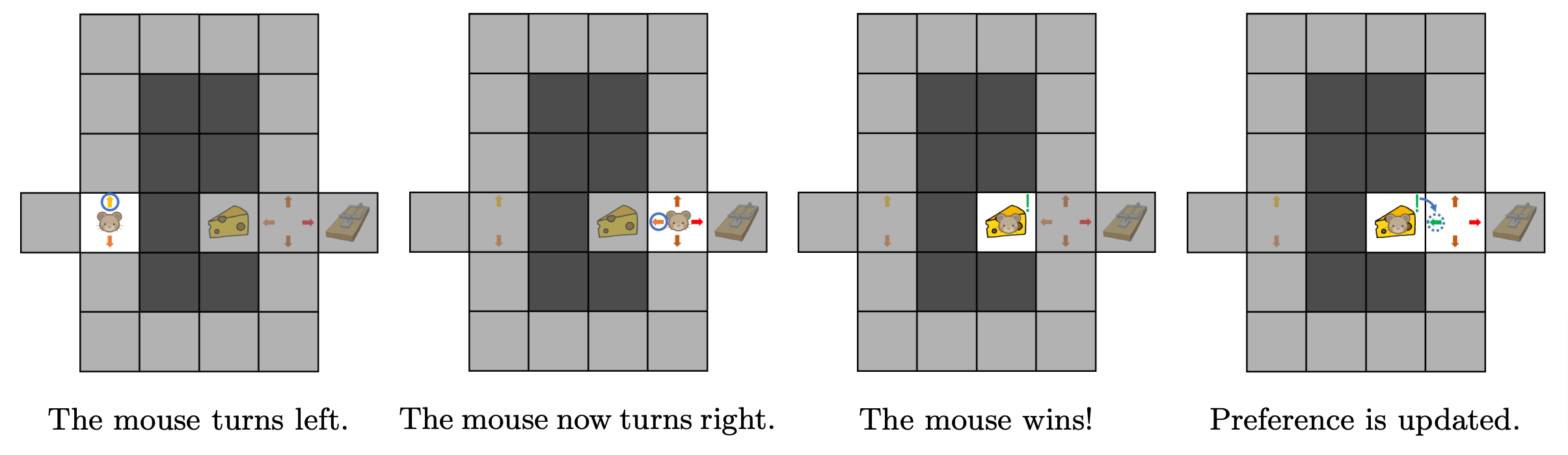Figure 4. Second episode.

The mouse can of course propagate what it learns at an intermediate position i.e. the second turn back to an earlier position i.e. the first turn. By doing so, it can associate early actions with their long-term consequences: turning left at first is a good choice, because it eventually leads to the cheese. Such a propagation of information is illustrated in Figure 5.

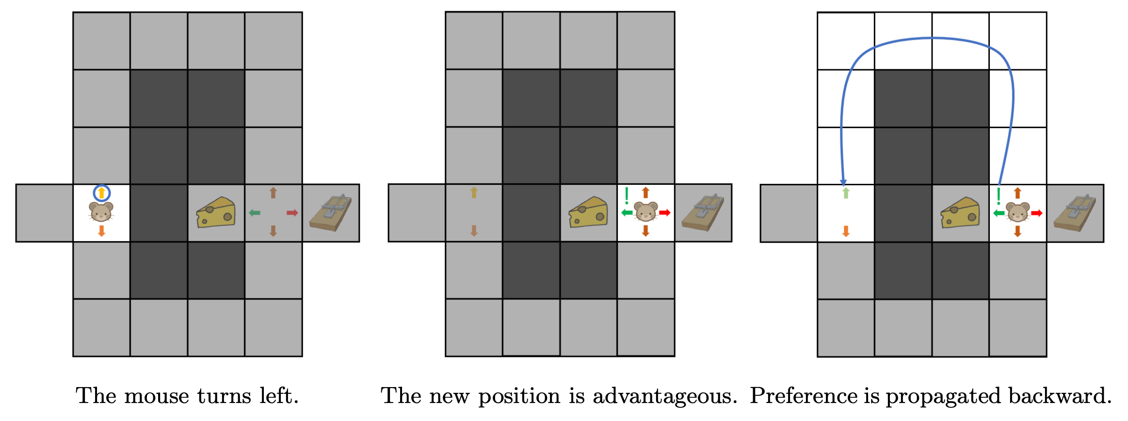Figure 5. Preference is propagated backward.

At this point, the mouse has learnt a reasonably good behaviour and may choose to stick to it. Yet, this behaviour could be further improved, as turning right on the first turn would give a shorter path to the cheese.

One way to improve the behaviour is for the mouse to explore: for instance, rather than follow its preferences at each action, the mouse has a small chance of moving in a direction that is not the preferred one. Thus, as the mouse keeps exploring the maze, it will eventually choose to turn right at the first turn and update its behaviour as shown in Figure 6. Therefore, the mouse has learnt the best behaviour to follow.

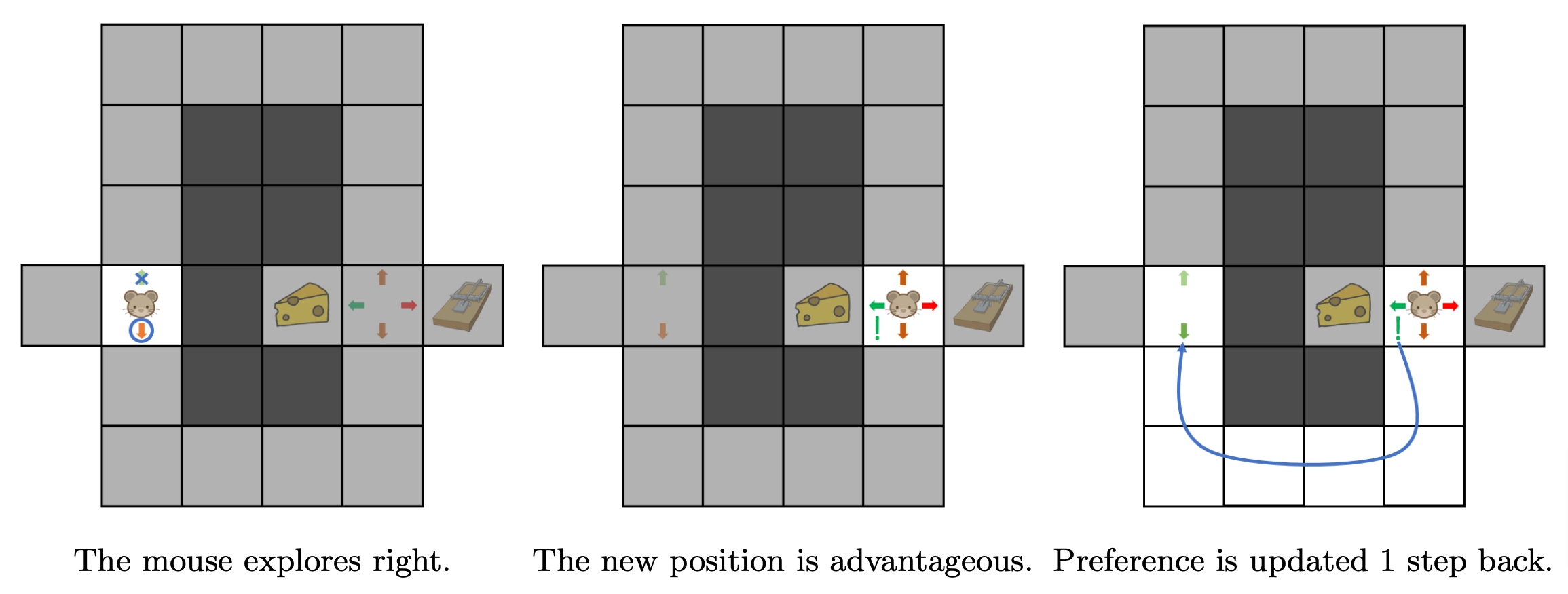
Figure 6. The importance of exploration.

This example outlines some essential features of RL:
• Having a behaviour that maps states to actions (called a policy in the literature);
• Evaluating this behaviour by assessing the corresponding cumulative reward;
• Using this evaluation to update the policy.

The mapping between (state, action) pairs to resulting cumulative rewards (i.e. the coloured arrows) is the action-value-function. The evaluation step uses a previous guess for this action-value-function to come up with a better guess, as in figure 5. Lastly, exploration allows to try and discover better behaviours.

The strategy followed by our mouse is an algorithm called $Q-$ learning. More details on it can be found in Carlos Esteve’s blog post “Q-learning for finite-dimensional problems”.

Reinforcement learning for optimal control

We can now understand why RL is an attractive option to tackle optimal control problems:
1. It proceeds by trial and error through mere interactions with the system, removing the need for an explicit mathematical model;
2. Deciding how to act at any given moment is computationally inexpensive;
3. The amount of exploration can be set to achieve a good compromise between testing only a small subset of possible behaviours and finding the best possible one. This, in a way, mitigates the curse of dimensionality.

To illustrate how RL can be used to control a mechanical system, we apply $Q-$ learning on a very simple problem as in Figure 7. A cart starts randomly in position $x_0 \in [-1, 0]$ with null velocity, and we wish to apply a minimal force to make it stop as possible to a target position $x_f = 0$ at time $T=1$ . This is quite similar to a satellite that we would want to bring into orbit.

Denoting $x$ the position of the cart over time, $\dot{x}$ its velocity and $\mathcal{U} = L^2([0, T], \mathbb{R})$ the set of admissible controls, this can be formulated as an optimal control problem:

$\underset{\mathbf{u} \in \mathcal{U}}{\mathrm{minimize}\,} \lambda_P \mathbf x(T)^2 + \lambda_V \dot{\mathbf x}(T)^2 + \int_0^T \mathbf u(t)^2 \, \mathrm{d} t$

with $\lambda_P,\, \lambda_V > 0$ two parameters setting the relative importance of the three evaluation criteria: reaching $x_f=0$ at time $T$ , stopping there (i.e., having zero velocity), and using as little force as possible. Note, then, that an optimal control may not necessarily bring the cart exactly in $0$ at final time. One may want to identify the equations that rule the motion, but we will assume they are unknown.

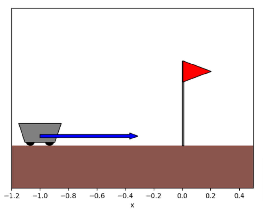Figure 7. The cart problem.

Discretizing this problem with time steps $(t_0=0, \dots, t_N=T)$ with $N \in \mathbb{N}^*$ , we can formulate it as an RL problem where:
• the state is the position $x_n$ and the velocity $\dot x_n$ at time $t_n$ , for $n \in \{0, \dots, N\}$ ;
• the action is the constant force $u_n$ applied over the time interval $[t_n, t_{n+1})$ , for $n \in \{0, \dots, N-1\}$ ;
• the reward is $- u_n^2$ for $n \in \{0, \dots, N-1\}$ , and $-\lambda_P \mathbf x(T)^2 - \lambda_V \dot{\mathbf x}(T)^2$ at the final time-step.

In this instance we use a more elaborate algorithm than $Q-$ learning, called Proximal Policy Optimization [2]. It relies on the same idea of having a policy, evaluating it and updating the policy using this evaluation, with a compromise to find on the amount of exploration. In this case however, the policy and the value-function are implemented as deep neural networks.

The experiment is carried out with $N=30$ , $\lambda_P = 200$ and $\lambda_V = 50$ . Before any training, the policy is set arbitrarily, and the cart doesn’t move. Then the agent trains through many episodes of this problem from random initial positions $x_0$ . After training, the agent has learnt to smoothly direct the cart to the flag, as shown in animation 8. Figure 9 compares the performance of the RL agent with the optimal solution found analytically. In this simple instance, the agent achieves a total cost that is $6.3\%$ larger than the optimum. Lastly, figure 10 shows the performance of the algorithm through training: every $1000$ time-steps, the agent is tested on $50$ episodes and the mean and standard deviation of the resulting costs make one point of the plot.

The same ideas can be used to control much more complicated systems. Those interested in learning more about this are referred to P. Garnier’s review article [1], which covers a range of successful applications of RL to control of fluid flows. This article also discusses some inherent challenges of RL, such as the large amount of training iterations needed to converge to an optimal behaviour.

Figure 8a. Before training.

Figure 8b. After training.

Figure 8. Trajectory of the cart obtained before and after training the agent for $x_0=-0.9$ .

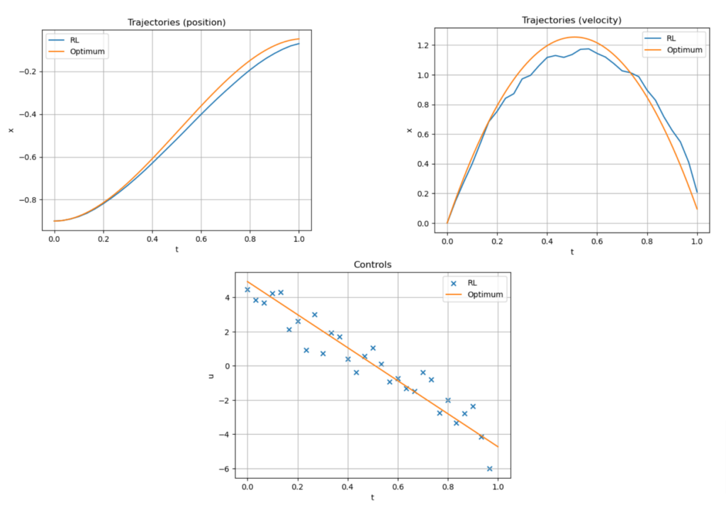Figure 9. Trajectory and control given by the trained RL agent for $x_0 = -0.9$ .

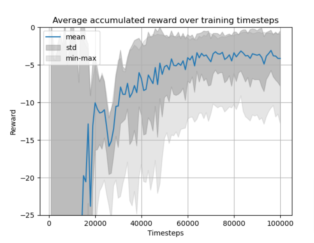Figure 10. Training curve for the RL agent.

GitHub Repository

Download resources from our FAU DCN-AvH GitHub, at: https://github.com/DCN-FAU-AvH/RL-cart/tree/main

Requirements

To run the code, it is advised to create a new virtual Python environment and to install Jupyter.

Then, the required libraries are listed in the requirements.txt file of each project folder. To install them, simply enter the corresponding folder and run
pip install -r requirements.txt

References

[1] P. Garnier, J. Viquerat, J. Rabault, A. Larcher, A. Kuhnle, and E. Hachem. A review on deep reinforcement learning for fluid mechanics. Computers & Fluids, 225:104973, July 2021.
[2] J. Schulman, F. Wolski, P. Dhariwal, A. Radford, and O. Klimov. Proximal Policy Optimization algorithms. ArXiv:1707.06347, 2017.
[3] R. S. Sutton and A. G. Barto. Reinforcement learning: An introduction, 2nd ed. The MIT Press, Cambridge, MA, US, 2018.