
Stability results for the KdV equation with time-varying delay

Introduction
The Korteweg-de Vries equation (KdV), is a third-order nonlinear one-dimensional equation given by y_{t}+y_{x}+y_{xxx}+yy_{x}=0. It was introduced in [6] to model the propagation of long water waves in a channel. In the last few years, the controllability and stabilization properties of the KdV have been very studied; see [3, 9] for a complete introduction of these problems.
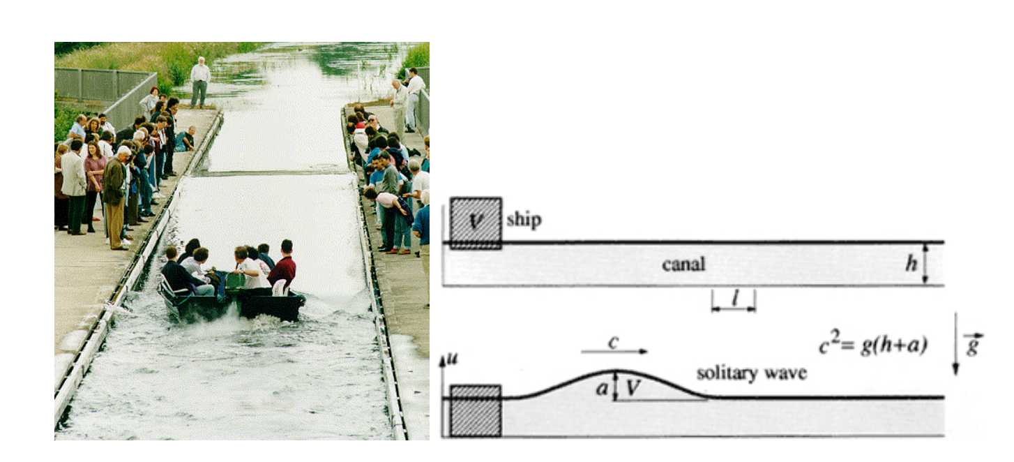
FIGURE 1. Solitary waves.
In this post, we are interested in the effect of a time-delay in the boundary stabilization of the KdV equation. Time delay phenomena appear in many applications, for example in biology, mechanics or engineering. Delays terms are unavoidable in practice due to measurement lag, analysis time, or computation time. Very active research has developed recently on stability problems of partial differential equations with delay. It is well known that even a small delay in the feedback mechanism can destabilize a system, see for example [4]. But a delay term can also improve the performance of the system [1].
1 Boundary time-varying delay
In this post inspired by [2], we are going to consider the following system
\left\{\begin{array}{ll} y_{t}+y_{x}+y_{xxx}+yy_{x}=0,& t>0, \ x \in (0,L), \\ y(0,t)=y(L,t)=0, &t>0, \\ y_{x}(L,t)=\alpha y_{x}(0,t)+\beta y_{x}(0,t-\tau(t)), &t>0, \\ y(x,0)=y_{0}(x), & x \in (0,L), \qquad \qquad (KdVd) \\ y_{x}(t-\tau(0),0)=z_{0}(t-\tau(0)),\quad 0 \lt t \lt \tau(0), \end{array}\right.
where \tau is the delay function which satisfies the following conditions
0 \lt \tau_{0}\leq \tau(t)\leq M,\qquad \forall t\geq0,\qquad(1) \\ \dot{\tau}(t)\leq d \lt 1,\qquad \forall t\geq0, \qquad \qquad (2)
where 0\leq d \lt 1, and
\tau \in W^{2,\infty}([0,T]),\qquad \forall T>0.\qquad \qquad (3)
Assume that \alpha, \beta, d in (KdVd) are real constants satisfying
\begin{gathered} \text{The matrix } \Phi_{\alpha,\beta}=\begin{pmatrix}\alpha^{2}-1+|\beta| & \alpha\beta \\ \alpha\beta & \beta^{2}+|\beta|(d-1)\end{pmatrix} \text{is definite negative. \qquad \qquad (4)} \end{gathered}
Let H=L^{2}(0,L)\times L^{2}(0,1) and define the energy of (KdVd) by
E(t)=\frac12 \displaystyle{\int_{0}^{L}}y^{2}(x,t)dx+\frac{|\beta|}{2}\,\tau(t)\displaystyle{\int_{0}^{1}}y_x^{2}(0,t-\tau(t)\rho)d\rho.\qquad \qquad (5)
The main result of this post is the following one
Theorem 1.1 (PVT [8]).
Suppose that (1)-(4) are satisfied and that L \lt \pi\sqrt{3}. Then, there exists r>0 such that, for every (y_{0},z_{0}) \in H satisfying \|(y_{0},z_{0})\|_{H}\leq r, we have E(t)\leq Ce^{-2\gamma t}E(0), \forall t>0, where, for \mu_{1} and \mu_{2} small enough,
\gamma \leq \min \bigg\{ \dfrac{(9\pi^{2}-3L^{2}-2L^{3/2}r\pi^{2})\mu_{1}}{3L^{2}(1+2L\mu_{1})},\dfrac{(1-d)\mu_{2}}{M(2\mu_{2}+|\beta|)} \bigg\}.
2 Well-posedness ideas
In this part, we focus in the study of linearization around 0 of (KdVd), that is
\left\{\begin{array}{l} y_{t}+y_{x}+y_{xxx}=0,\quad t>0, \ x \in (0,L), \\ y(0,t)=y(L,t)=0,\quad t>0, \\ y_{x}(L,t)=\alpha y_{x}(0,t)+\beta y_{x}(0,t-\tau(t)),\quad t>0, \\ y(x,0)=y_{0}(x),\quad x \in (0,L), \\ y_x(0,t-\tau(0))=z_{0}(t-\tau(0)), \quad 0 \lt t \lt \tau(0).\qquad \qquad (6) \end{array}\right.
Now, we introduce z(\rho,t)=y_{x}(0,t-\tau(t)\rho) for \rho \in (0,1) and t>0. Then, z verifies the following transport equation
\left\{\begin{array}{l} \tau(t)z_{t}(\rho,t)+(1-\dot{\tau}(t)\rho)z_{\rho}(\rho,t)=0,\, t>0,\, \rho \in (0,1), \\ z(0,t)=y_{x}(0,t),\quad t>0, \\ z(\rho,0)=z_{0}(-\tau(0)\rho),\quad \rho \in (0,1). \end{array}\right.
Define U=(y, z)^T, then we can see (6) in the following setting
\left\{\begin{array}{ll} U_{t}(t)=\mathcal{A}(t)U(t),\qquad t>0, & \mathcal{A}(t)\begin{pmatrix}y \\ z \end{pmatrix}=\begin{pmatrix}-y_{x}-y_{xxx}\\ \dfrac{\dot{\tau}(t)\rho-1}{\tau(t)}z_{\rho} \end{pmatrix},\qquad \qquad (7)\\ U(0)=(y_{0}, z_{0}(-\tau(0)\cdot))^T=:U_{0}. & \end{array}\right.
with
\begin{gathered} D(\mathcal{A}(t))=\left\{(y,z) \in \left(H^{3}(0,L)\cap H_{0}^{1}(0,L)\right)\times H^{1}(0,1), \ z(0)=y_{x}(0),\right. \\ \left. y_{x}(L)=\alpha y_{x}(0)+\beta z(1)\right\}.\end{gathered}
Note that, D(\mathcal{A}(t))=D(\mathcal{A}(0)), t>0. We are in the framework of Constant domain system (CD-system) and we can follow [5], to derive a well-posedness result of (6). Finally, the well-posedness of (KdVd) is obtained using fixed point arguments.
3 Exponential stability
Consider the Lyapunov candidate
V(t)=E(t)+\mu_{1}V_{1}(t)+\mu_{2}V_{2}(t),
where \mu_{1}, \mu_{2}>0 and
V_{1}(t)=\int_{0}^{L}xy^{2}(x,t)dx, \quad V_{2}(t)=\tau(t)\int_{0}^{1}(1-\rho)y_x^{2}(0,t-\tau(t)\rho)d\rho.
For \mu_{1}, \mu_{2}>0 small enough we can show
\begin{gathered} \dot{V}(t)+2\gamma V(t)\leq \left(\frac{L^{2}}{\pi^{2}}(\mu_{1}+\gamma+2L\mu_{1}\gamma)+\dfrac{2}{3}L^{3/2}r\mu_{1}-3\mu_{1}\right)\int_{0}^{L}y^{2}_{x}dx\\ +(\gamma|\beta|M+2\mu_{2}\gamma M-\mu_{2}(1-d))\int_{0}^{1}y_x^{2}(0,t-\tau(t)\rho)d\rho. \end{gathered}
Now, following [2], as L \lt \pi\sqrt{3}, it is possible to choose r small enough to have r \lt \frac{3(3\pi^{2}-L^{2})}{2L^{3/2}\pi^{2}}. Then, we can choose \gamma>0 such that \dot{V}(t)+2\gamma V(t)\leq 0 and hence V(t)\leq V(0)e^{-2\gamma t} for all t>0. Therefore, we obtain the exponential decay.
Numerical Simulations
Consider L=1, T=10, initial conditions y_{0}(x)=0.5(1-\cos(2\pi x)), z_{0}(\rho)=-0.5\sin(2\pi\rho) and delay \tau(t)=d(1.5+\sin(t)).
For Figure 2 we use \alpha=0.1 and \beta=0.1. We can observe how the decay rate depends on the size of d. In particular, in the case d=1.3 which not satisfies (2), the energy is not decreasing.
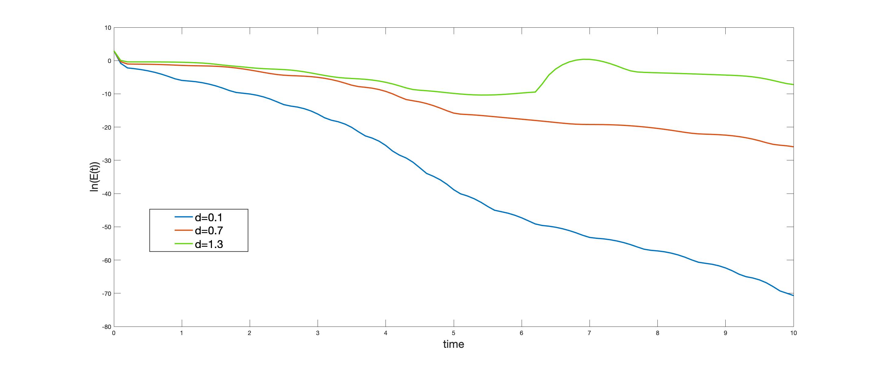
FIGURE 2. Time-evolution of t \mapsto \ln(E(t)) for different values of d.
In Figure 3 we present a comparison between the action of time-varying delay and constant delay. We see how the energy associates to time-varying delay is oscillating between the associated to \tau_{max}=2.5d and \tau_{min}=0.5d.
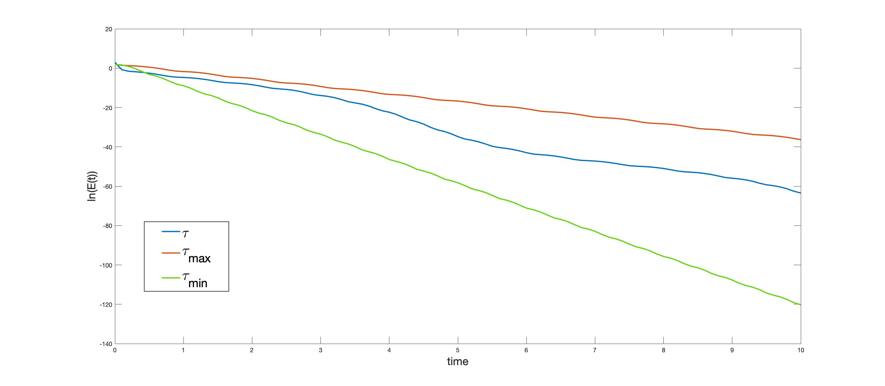
FIGURE 3. Time-evolution of t \mapsto \ln(E(t)) in the case of constant and varying boundary delay.
5 Perspectives and Extensions
Following the works, [7,10], similar results can be obtained for the system
\begin{cases} y_{t}+y_{x}+y_{xxx}+yy_{x}+a(x)y(x,t)+b(x)y(x,t-\tau(t))=0,& t>0, \ x \in (0,L), \\ y(0,t)=y(L,t)=y_{x}(L,t)=0, &t>0, \\ y(x,0)=y_{0}(x), & x \in (0,L), \\ y(x,t-\tau(0))=z_{0}(x,t-\tau(0)), & 0\lt t \lt \tau(0), \ x \in (0,L), \end{cases}
Now we give some possible extension in this topic:
• Take in our results, time-varying delay that could vanish at some time 0\leq \tau(t)\leq M.
• Delay in the nonlinearity y(t-h,x)y_{x}(t,x) or y(t,x)y_{x}(t-h,x).
• Space-time varying delay \tau(t,x).
• Other equations as Kawahara (fifth order KdV).
References
[1] C. Abdallah, P. Dorato, J. Benites-Read, and R. Byrne. Delayed positive feedback can stabilize oscillatory systems. In 1993 American Control Conference, pages 3106–3107. IEEE, 1993.[2] L. Baudouin, E. Crépeau, and J. Valein. Two approaches for the stabilization of nonlinear KdV equation with boundary time-delay feedback. IEEE Transactions on Automatic Control, 64(4):1403–1414, Apr. 2019.
[3] E. Cerpa. Control of a Kortewegde Vries equation: a tutorial. Mathematical Control & Related Fields, 4(1):45, 2014.
[4] R. Datko. Not all feedback stabilized hyperbolic systems are robust with respect to small time delays in their feedbacks. SIAM J. Control Optim., 26(3):697–713, 1988.
[5] T. Kato. Linear evolution equations of “hyperbolic” type. J. Fac. Sci. Univ. Tokyo Sect. I, 17:241–258, 1970.
[6] D. Korteweg and G. de Vries. On the change of form of long waves advancing in a rectangular channel, and a new type of long stationary wave. Phil. Mag, 39:422–443, 1895.
[7] H. Parada, E. Crépeau, and C. Prieur. Delayed stabilization of the Korteweg–de Vries equation on a star-shaped network. Mathematics of Control, Signals, and Systems, pages 1–47, Feb 2022.
[8] H. Parada, C. Timimoun, and J. Valein. Stability results for the KdV equation with time-varying delay. Submitted, Oct. 2022.
[9] L. Rosier and B.-Y. Zhang. Control and stabilization of the Korteweg-de Vries equation: recent progresses. Journal of Systems Science and Complexity, 22(4):647–682, 2009.
[10] J. Valein. On the asymptotic stability of the Kortewegde Vries equation with time-delayed internal feedback. Mathematical Control and Related Fields, 12(3):667–694, 2022.
|| Go to the Math & Research main page


