
3−wave turbulence kinetics: Numerical approach for energy cascading
 Arijit Das
This post provides an overview of the results presented in the paper “Numerical schemes for a fully nonlinear coagulation-fragmentation model coming from wave kinetic theory” by Arijit Das and Minh-Binh Tran [1].
1. Introduction
The theory of wave turbulence has been shown to play important roles in a vast range of physical and mechanical examples including inertial waves due to rotation, Alfvén wave turbulence in the solar wind, waves in plasmas of fusion devices, and many others. The common theme of all kind of wave kinetic models is the representation of energy distribution among weakly interacting waves. The general form of 3-wave kinetic equations [2, 3, 4] reads
\begin{aligned} \partial_tf(t,p) =& \iint_{\mathbb{R}^{2d}} \Big[ R_{p,p_1,p_2}[f] - R_{p_1,p,p_2}[f] - R_{p_2,p,p_1}[f] \Big] \text{d} p_1 \text{d} p_2, \ f(0,p) \ = \ f_0(p), \hspace{1cm}(1.1) \end{aligned}
where f(t,p) is the wave density at wavenumber p\in \mathbb{R}^d, f_0(p) is the initial condition. Moreover,
R_{p,p_1,p_2} [f]:= |V_{p,p_1,p_2}|^2\delta(p-p_1-p_2)\delta(\omega -\omega_{1}-\omega_{2})(f_1f_2-ff_1-ff_2), \hspace{1cm}(1.2)
with the short-hand notations f = f(t,p), \omega = \omega(p) and f_j = f(t,p_j), \omega_j = \omega(p_j), for p, p_j, j\in\{1,2\}. The quantity \omega(p) is the dispersion relation of the waves. For a deeper physical understanding, we refer to the comprehensive works in [5, 6, 7].
In a related context, Coagulation-fragmentation kinetic equation describes the behavior of particles that coagulate or fragment due to the mutual interactions or some external force. Coagulation-fragmentation kinetics plays a crucial role in wave turbulence theory. There is a conceptual analogy between coagulation-fragmentation kinetics and 3-wave kinetic models: the transfer of energy between scales in wave turbulence is analogous to the transfer of mass between clusters in coagulation processes. This observation offers a quantitative bridge between the two fields. Building on this analogy, Connaughton [8] proposed an approximation of the 3-wave kinetic equations (1.1)-(1.2) using a nonlinear coagulation-fragmentation model as follows:
\begin{aligned} \frac{\partial N_{\omega}}{\partial t} = \mathcal{Q}\left[N_\omega\right](t):=\mathcal{Q}\left[N_\omega\right](t) = S_1\left[N_{\omega}\right] - S_2\left[N_{\omega}\right] - S_3\left[N_{\omega}\right], ~ \omega \in \mathbb{R}_+, ~ N_\omega(0)= N_\omega^{in}, \end{aligned}
with
S_1\left[N_{\omega}\right] = \int_{0}^{\omega}K_1(\omega-\mu,\mu)N_{\omega-\mu}N_{\mu}\text{d} \mu - \int_{\omega}^\infty K_1(\mu-\omega,\omega)N_{\mu-\omega}N_{\omega}\text{d} \mu - \int_{0}^{\infty} K_1(\omega,\mu) N_\omega N_{\mu}\text{d} \mu \\
S_2\left[N_{\omega}\right] = - \int_{0}^{\omega} K_2(\mu,\omega-\mu)N_\omega N_{\mu}\text{d} \mu + \int_{\omega}^{\infty} K_2(\omega,\mu-\omega)N_{\mu-\omega}N_{\mu}\text{d} \mu+ \int_{0}^{\infty} K_2(\omega,\mu) N_\omega N_{\omega+\mu}\text{d} \mu,\\
S_3\left[N_{\omega}\right] = -\int_{0}^{\omega}K_3(\mu,\omega-\mu)N_\omega N_{\omega-\mu}\text{d} \mu + \int_{\omega}^{\infty} K_3(\omega,\mu-\omega)N_{\omega}N_{\mu}\text{d} \mu+ \int_{0}^{\infty}K_3(\omega,\mu) N_{\mu} N_{\omega+\mu}\text{d} \mu.
The wave frequency spectrum N_\omega is defined such that \int_{\omega_{1}}^{\omega_{2}}N_\omega\text{d}\omega represents the total wave action in the frequency band \left[\omega_{1},\omega_{2}\right]. To analyze solutions to the nonlinear coagulation-fragmentation model (1.3), we define the p-th moment as:
M_p(t) = \int_{0}^{\infty} \omega^p N_\omega(t)\text{d} \omega,\quad\text{for all}\quad p\ge 0.
In this regard, the total number of wave N and total wave energy E can be obtained from the zeroth and first moments, respectively.
Also, the nonnegative homogeneous functions K_i(\omega,\mu) (i=1,2,3) represent the wave interaction kernels. Among these kernels, K_1 facilitates the forward transfer of energy, while K_2 and K_3 are associated with the back-scattering of energy.
2. Formulation of finite volume scheme
We first truncate the computational domain \mathcal{D}= \left[0,R\right] consider the truncated form of the fully nonlinear coagulation-fragmentation model equation as
\frac{\partial N_{\omega}}{\partial t} = S^{nc}_1\left[N_{\omega}\right] - S^{c}_2\left[N_{\omega}\right] - S^{c}_3\left[N_{\omega}\right], \qquad \omega \in \mathbb{R}_+. \hspace{1cm}(2.1)
Here
S^{nc}_1\left[N_{\omega}\right] = \int_{0}^{\omega}K_1(\omega-\mu,\mu)N_{\omega-\mu}N_{\mu}\text{d} \mu - 2 \int_{0}^{R} K_1(\omega,\mu) N_\omega N_{\mu}\text{d} \mu,\\
S^{c}_2\left[N_{\omega}\right] = - \int_{0}^{\omega} K_2(\mu,\omega-\mu)N_\omega N_{\mu}\text{d} \mu + \int_{\omega}^{R} K_2(\omega,\mu-\omega)N_{\mu-\omega}N_{\mu}\text{d} \mu+ \int_{0}^{R-\omega} K_2(\omega,\mu) N_\omega N_{\omega+\mu}\text{d} \mu,\\
S^{c}_3\left[N_{\omega}\right] = -\int_{0}^{\omega}K_3(\mu,\omega-\mu)N_\omega N_{\omega-\mu}\text{d} \mu + \int_{\omega}^{R} K_3(\omega,\mu-\omega)N_{\omega}N_{\mu}\text{d} \mu + \int_{0}^{R-\omega}K_3(\omega,\mu) N_{\mu} N_{\mu+\omega}\text{d} \mu.
For the numerical scheme, let us discretize the computational domain \mathcal{D} into I number of cells with the limits 0 to R \lt \infty. Moreover, each of the i-th sub interval for i\in \{0,1,2,...,I\}, is denoted by \Lambda_i:= \left[\omega_{i-1/2},\omega_{i+1/2}\right] and the cell representative of the i-th cell is given by \omega_{1/2}=0, \quad \omega_{I^h+1/2}=R, \quad \omega_i = \frac{\omega_{i-1/2}+\omega_{i+1/2}}{2}.
Furthermore, introduce the bound \Delta\omega and \Delta\omega_{min} as follows
\Delta\omega_{min}\le \omega_{i+1/2}-\omega_{i-1/2}:=\Delta \omega_i \le \Delta\omega.
Moreover, for a fully discrete formulation, the time domain need to discretized. To discretize the time variable t, we split the time interval [0,T] into N subintervals \tau_n:=[t_n,t_{n+1}), \text{for} \quad n \in \{0,1,...,N-1\}, with t_n=n\Delta t and N\Delta t=T.
The above discretization of volume variable x and time variable t leads to the discretize form of the collision kernel as follows; for i,j \in \{1,...,I\}
\begin{aligned} K_1(u,v) \approx K^1_{i,j}, K_2(u,v) \approx K^2_{i,j}, K_3(u,v) \approx K^3_{i,j}\quad\text{when} \quad u\in \Lambda_i, ~v\in \Lambda_j. \end{aligned}
The numerical values approximating N_i(t) at time t_n is denoted by N_i^n. Therefore, the wave density function can be represented as
\begin{aligned} N_\omega \approx \sum_{i=1}^{I} N_i^n\Delta \omega_i \delta\left(\omega-\omega_i\right). \end{aligned}
To formulate the numerical scheme, we also need to the following sets of indices as
\begin{aligned} &\mathcal{I}_{j,k}^i:= \{(j, k) \in \mathbb{N}\times \mathbb{N}: \omega_{i-1/2} \le \omega_j +\omega_k \lt \omega_{i+1/2}\},\\ & \mathcal{J}_{j,k}^i := \{(j, k) \in \mathbb{N}\times \mathbb{N}: \omega_{i-1/2} \le \omega_j - \omega_k \lt \omega_{i+1/2}\}. \end{aligned}
Using the aforementioned notation of the index sets with the approximation (2.2), the numerical Finite Volume Scheme (FVS) can be written as follows:
\begin{aligned} N_i^{n+1}=N_i^n + \Delta t^n &\left(\sum_{(j,k)\in \mathcal{I}_{j,k}^i} K^1_{j,k} N_j^n N_k^n \frac{\Delta \omega_j \Delta \omega_k}{\Delta \omega_i} -2 \sum_{j=1}^{I} K^1_{i,j} N_i^n N_j^n \Delta \omega_j \right. \\ &\left. + \sum_{j=i+1}^{I} \left(K^2_{j-i,i}+K^3_{j-i,i}\right)N^n_i N^n_j \Delta \omega_j-\sum_{j=1}^{i-1} \left(K^2_{i-j,j}+K^3_{i-j,j}\right)N^n_i N^n_j \Delta \omega_j \right. \\ &\left.\quad + \sum_{(j,k)\in \mathcal{J}_{j,k}^i} \left(K^2_{j-k,k}+K^3_{j-k,k}\right) N_j^n N_k^n \frac{\Delta \omega_j \Delta \omega_k}{\Delta \omega_i} \right) . \end{aligned}
New formulation of the energy conserving scheme
Since our aim of the FVS is to conserve the total energy of the system, however, the scheme (2.3) only predict the zeroth order moment but not for the conservation of the total energy of the system. However, this can be achieved by introducing the suitable weight functions into the formulation. Hence, the expression of the energy conserving scheme takes the following form:
\begin{aligned} N_i^{n+1}=N_i^n + \Delta t^n &\left(\sum_{(j,k)\in \mathcal{I}_{j,k}^i} K^1_{j,k} N_j^n N_k^n \frac{\Delta \omega_j \Delta \omega_k}{\Delta \omega_i} \alpha_{j,k} -2 \sum_{j=1}^{I} K^1_{i,j} N_i^n N_j^n \Delta \omega_j \right. \\ &\left. + \sum_{j=i+1}^{I} \left(K^2_{j-i,i}+K^3_{j-i,i}\right)N^n_i N^n_j \Delta \omega_j-\sum_{j=1}^{i-1} \left(K^2_{i-j,j}+K^3_{i-j,j}\right)N^n_i N^n_j \Delta \omega_j \beta_{i,j} \right. \\ &\left.\quad + \sum_{(j,k)\in \mathcal{J}_{j,k}^i} \left(K^2_{j-k,k}+K^3_{j-k,k}\right) N_j^n N_k^n \frac{\Delta \omega_j \Delta \omega_k}{\Delta \omega_i} \right) . \hspace{1cm} (2.4) \end{aligned}
Where the weights \alpha_{j,k} are \beta_{i,j} are the weights responsible for the conservation of energy. The weights are defined as
\begin{aligned} \alpha_{j,k} := \left\{\begin{array}{ll} \frac{\omega_j + \omega_k}{\omega_i}, &\ \text{if}\quad \omega_j + \omega_k \le R, \\ 0 , &\ \text{otherwise}, \end{array}\right. \text{and}\quad \beta_{i,j}:= \left\{\begin{array}{ll} \frac{ 2\omega_j}{\omega_i}, &\ \text{if}\quad 0 \lt \omega_i, \omega_j \le R, \\ 0 , &\ \text{otherwise}. \end{array}\right. \end{aligned}
3. Numerical test
To test our numerical schemes, we will rely on the theoretical work [9], where they prove that the energy on the interval \left[0,\infty\right) is a non-increasing function in time.
They also decompose the energy of a solution g_\omega(t) = \omega N_\omega(t) at any time t as follows
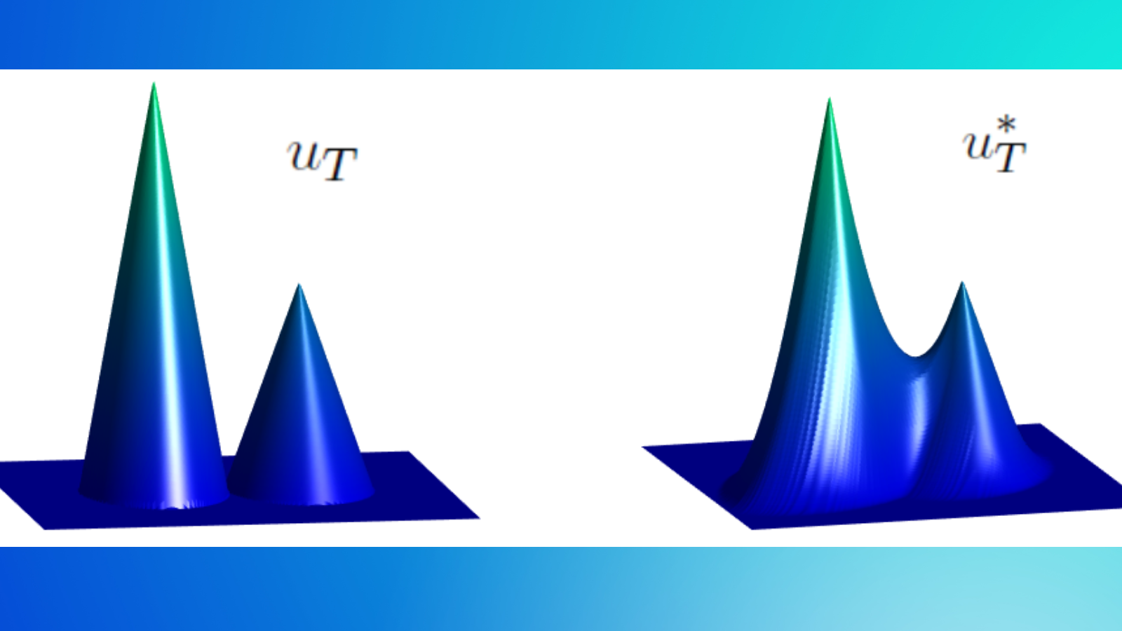
\begin{aligned} g_\omega(t) = \bar{g}_\omega(t) + \tilde{g}(t) \delta_{\{\omega=\infty\}}. \hspace{1cm} (3.1) \end{aligned}
Where the nonnegative function \bar{g} is the regular part and \tilde{g} be the singular part, which indicates that initially, the energy is concentrated in the regular part, and as time progresses, energy gradually accumulates at \{\omega=\infty\}. In this context, there exist a positive time t_1^\ast known as first blow-up time for which \tilde{g}(t) >0 for all t>t_1^\ast. Moreover, after the first blow-up time there exist infinitely many blow-up time represented by the sequence 0 \lt t_1^\ast \lt t_2^\ast \lt \cdot\cdot\cdot \lt t_n^\ast \lt \cdot\cdot\cdot, satisfying \bar{g}_\omega(t_1^\ast)> \bar{g}_\omega(t^\ast_2)>\cdot\cdot\cdot> \bar{g}_\omega(t_n^\ast)>\cdot\cdot\cdot ~\text{and}~~ \tilde{g}(t_1^\ast) \lt \tilde{g}(t_2^\ast) \lt \cdot\cdot\cdot \lt \tilde{g}(t_n^\ast) \lt \cdot\cdot\cdot.
If we consider \chi_{[0,R]}(\omega) be a cutt-off function of \omega in the finite domain [0,R], the equivalent form of the multiple blow-up time phenomena can be represented for arbitrary parameter R,
\begin{aligned} \int_{\mathbb{R}_+}\chi_{[0,R]}(\omega) \omega N_\omega \text{d} \omega \le \mathcal{O}\left(\frac{1}{\sqrt{t}}\right), ~\text{as}~ t \longrightarrow\infty,~\text{and}~ \lim\limits_{t \to \infty} N_\omega(t) \chi_{[0,R]}(\omega) = 0. \end{aligned}
Our finite volume scheme allows for the numerical observation of the multiple blow-up time phenomenon, t_1^\ast \lt t_2^\ast \lt \cdot\cdot\cdot \lt t_n^\ast \lt \cdot\cdot\cdot, as well as the verification of the energy decay rate estimate given by (3.2) for the fully nonlinear coagulation-fragmentation model (1.3).
Among the several test problems in [1], here we consider an analytical initial condition, N_\omega^{in} = 1.25 \omega e^{-100\left(\omega-0.25\right)^2}, \omega\ge 0 with the collision kernels K_1(\omega,\mu)= (\omega\mu)^\theta, K_2(\omega,\mu)= (\omega\mu)^\gamma, and K_3(\omega,\mu) = (\omega\mu)^\delta, where \theta, \gamma and \delta \ge 0. We begin implementing the FVS (2.3) with the specific case \theta=\gamma=\delta and truncation parameter R=100. The time evolution of the first three moments M_1(t), M_2(t) and M_3(t) is plotted for different degrees of the collision kernel: \theta= 1, 0.85, 0.75 in Figure (3.2), which also support the theoretical result (3.2).
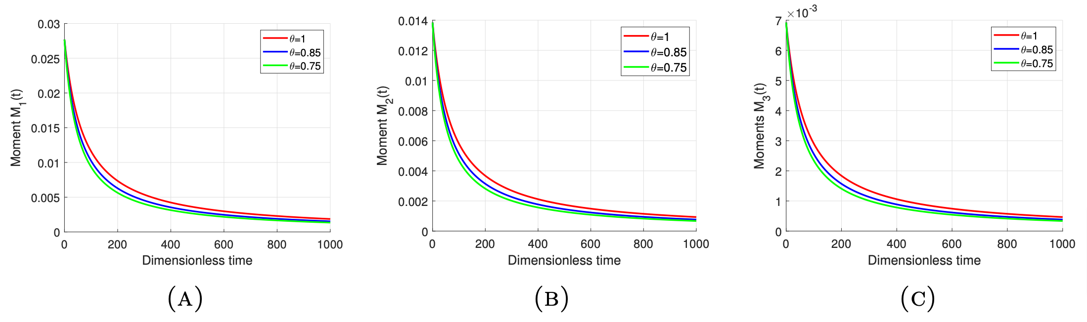
Figure 1. Time evolution of the (A) first, (B) second, and (C) third moments for different degrees of homogeneity \theta with the same truncation parameter R.
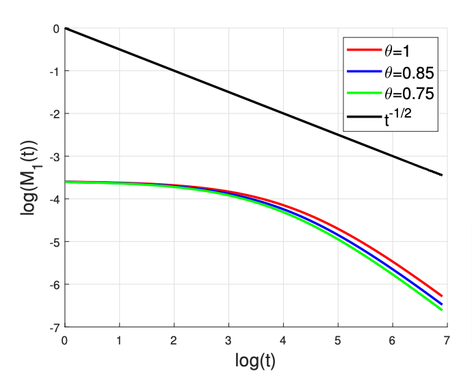
Figure 2. Decay of total energy for different values of \theta in logarithmic scale.
Figure 2 demonstrates that the theoretical result (3.2) is in good agreement with the numerical results, where the slope of the decay rate curve is below the slope line corresponding to \frac{1}{\sqrt{t}}.
To test the performance of our scheme for different collision kernels, we choose the collision kernels with \theta\ne \gamma\ne \delta and plot the time evolution of three different moments in Figure 3.
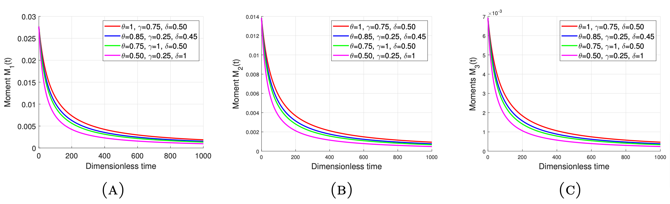
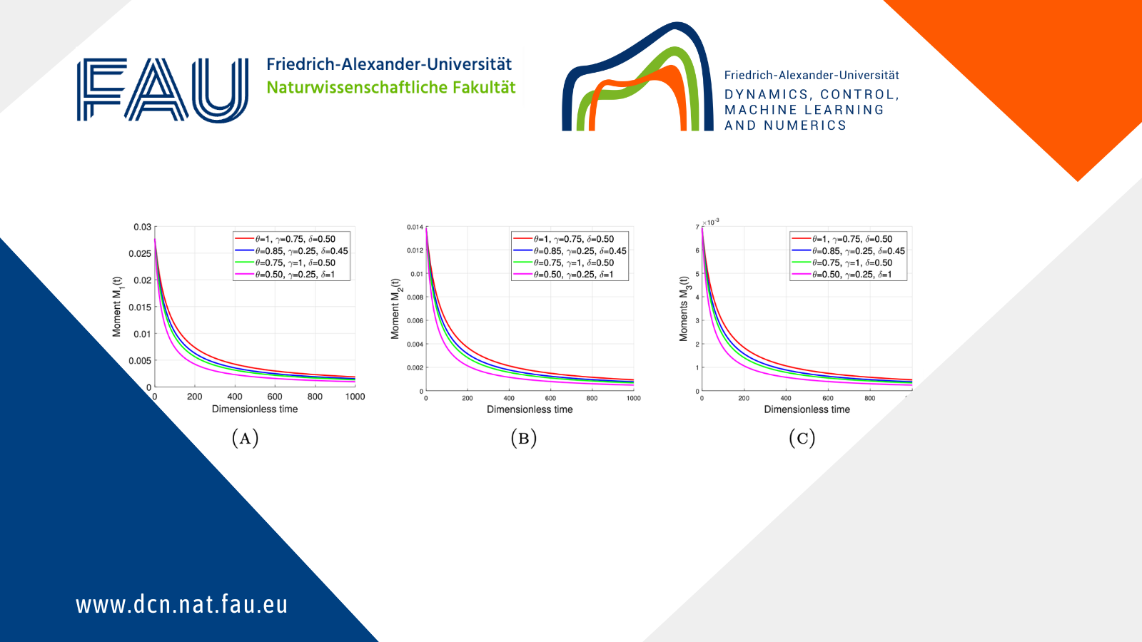
Figure 3. Time evolution of the (A) first, (B) second, and (C) third moments for different values of \theta, \gamma and \delta with the same truncation parameter R.
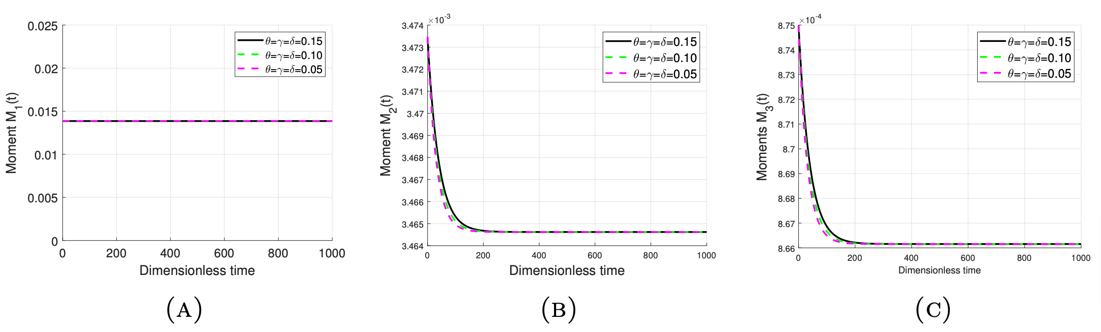
Figure 4. Time evolution of the (A) first, (B) second, and (C) third moments for different values of \theta with the same truncation parameter R.
To conserve the total energy, we have implemented our proposed weighted FVS (2.4) for the same initial data and set \theta=\gamma=\delta=0.15,0.10, 0.05 in Figure 4. From Figure 4a, we can see that our weighted FVS successfully conserves energy for a large time domain. Figures 4b and 4c depicted the other two moments show a tendency to stabilize after a short period of time.
References
[1] A. Das, M.-B. Tran, Numerical schemes for a fully nonlinear coagulation-fragmentation model coming from wave kinetic theory, arXiv preprint arXiv:2412.05402 (2024).[2] K. Hasselmann, On the non-linear energy transfer in a gravity-wave spectrum part 1. general theory, Journal of Fluid Mechanics 12 (4) (1962) 481–500.
[3] V. Zakharov, N. Filonenko, Weak turbulence of capillary waves, Journal of applied mechanics and technical physics 8 (5) (1967) 37–40.
[4] K. Hasselmann, On the spectral dissipation of ocean waves due to white capping, Boundary-Layer Meteorology 6 (1974) 107–127.
[5] S. Nazarenko, Wave turbulence, Vol. 825, Springer, 2011.
[6] Y. Pomeau, M.-B. Tran, Statistical physics of non equilibrium quantum phenomena, Springer, 2019.
[7] V. E. Zakharov, V. S. L’vov, G. Falkovich, Kolmogorov spectra of turbulence I: Wave turbulence, Springer Science & Business Media, 2012.
[8] C. Connaughton, A. C. Newell, Dynamical scaling and the finite-capacity anomaly in three-wave turbulence, Physical Review E—Statistical, Nonlinear, and Soft Matter Physics 81 (3) (2010) 036303.
[9] A. Soffer, M.-B. Tran, On the energy cascade of 3-wave kinetic equations: beyond kolmogorov–zakharov solutions, Communications in Mathematical Physics 376 (3) (2020) 2229–2276.