Network design and control: Shape and topology optimization for the turnpike property for the wave equation

Network design and control: Shape and topology optimization for the turnpike property for the wave equation

 

1 Introduction

We consider two optimal control problems. The first problem, denoted by (OCE), is an optimal control problem governed by an evolution equation. The second problem, denoted by (OCS), is the optimal control problem for the associated steady-state equation, obtained by reducing the evolution equation to its stationary counterpart. The optimal controls are given by the appropriate optimality systems. In order to justify the approximation of (OCE) by (OCS), we study the turnpike property of the pair (OCE)–(OCS). Several forms of the turnpike phenomenon have been studied in detail, for example, the exponential turnpike property and the interval turnpike property.

 

2 Optimal control problems on graphs

Let us consider the finite connected graph G=(V, \, E) where V=\{ P_j | j\in\cal {J}\} is the set of vertices and E=\{ E_i | i\in\cal {I}\} the set of edges. We consider the evolution equations on the edges of G. The dynamics of the edges are coupled by suitable node conditions, such as those of Kirchhoff type.
Therefore we assume that the edges correspond to curves \Omega_i in {\mathbb R}^1, {\mathbb R}^2, or {\mathbb R}^3. Define \Omega = \overline{ \cup_{ i\in\cal {I} } \Omega_i} . We are interested in control problems defined on G. The controls are denoted by v:=v(x) with x\in\Omega, and by u_T:=u_T(x,t) with x\in\Omega and t\in (0,T).

 
Static problem
The static state z:=z(v;x)=z(x) is determined by the state equation for

z\in H\, :\, a(z,\phi)=(\mathcal{B}(v),\phi)+ (f,\phi),\,\,\forall\phi\in H \,, \qquad (1)

where x\mapsto z(v;x) lives in the Hilbert space H. In typical applications, H is a Sobolev space.
We assume that the bilinear form a(\cdot,\cdot) is symmetric and coercive with a bounded linear operator \mathcal{B} from the space of controls to H and f\in H.

 
Evolution problem
We consider the evolution equation that governs the state denoted by y:=y(u;x,t)=y(x,t) in variational form for t\mapsto y(u;x,t):

\left( \frac{\partial^2 y}{\partial t^2}(t),\varphi \right) +a(y(t),\varphi)= (\mathcal{B}(u)(t),\varphi)+(F(t),\varphi), \qquad (2)

for all \varphi\in H and a.e. for t\in (0,T), along with the initial conditions y(0,x)=y^0(x) and y_t(0,x)=y^1(x). Here, H is the Hilbert space that contains the functions with H^1-regularity on the edges that are compatible with the node conditions that are prescribed on the vertices. Moreover, F(t)=f for all t\in (0, \, T).

 
Cost functionals
The simplest possibility is the quadratic cost with the appropriate choice of norms in Hilbert function spaces. For the static problem, it is

I(v)=\frac{1}{2}\| z-z^d\|_{L^2(\Omega)}^2+\frac{1}{2}\| v-v^d\|_{L^2(\Gamma)}^2\,. \qquad (3)

For the evolution problem, it is

J_T(u)=\frac{1}{2}\int_0^T\| y-y^d\|_{L^2(\Omega)}^2 + \gamma \, \|\partial_t( y-y^d)\|_{L^2(\Omega)}^2 dt+\frac{1}{2}\int_0^T\| u-u^d\|_{L^2(\Gamma)}^2dt, \qquad (4)

where \gamma \in (0, \, \infty). For simplicity, the control problems are considered without constraints.

 
Optimality system for the static problem
The optimality system for the static control problem is equivalent to the vanishing of the gradient for the cost, hence

\min_{v}\{ J(v) \}=J(\hat{v})

if the following optimality system is verified

\hat{z} \in H\, :\, a(\hat{z},\varphi)=(\mathcal{B}(\hat{v}),\varphi)+ (f,\varphi)\, ,\forall\varphi\in H , \qquad (5) \\ \hat{p}\in H\, :\, a(\hat{p},\phi)=(z_d-\hat{z},\phi)\, ,\forall\phi\in H , \qquad (6) \\ (v_d-\hat{v},v)_U=(\mathcal{B}^{\prime}(\hat{v})\cdot v,\hat{p})\, ,\forall v\in U . \qquad (7)

 
Optimality system for the evolution problem
We derive the optimality system for the optimal control problem with the evolution state equation. To this end, we introduce the Lagrangian

\mathcal{L}(u, y, \varphi)

with y\in L^2(0,T;H^1(\Omega)),
y_t\in L^2(Q), y(0)=y^0, and \varphi\in L^2(0,T;H^1(\Omega)),
\varphi_t\in L^2(Q), \varphi(T)=0.

 
Lemma 2.1
The optimality system for the optimal control problem governed by the evolution equation is verified for a.e. t\in(0,T):

(\hat{y}_{tt},\varphi)_{Q(T)} +\int_0^T a(\hat{y}(t),\varphi) \, dt = \int_0^T(L(\hat{u})(t),\varphi)_\Gamma \, dt +(F(t),\varphi)_{Q(T)}\,, \forall\varphi \in H(Q(T)), \qquad (8) \\ \hat{y}(0)=y^0,\,\, \hat{y}_t(0)=y^1, \qquad (9) \\ (\hat{p}_{tt},\varphi)_{Q(T)}+ \int_0^T a(\hat{p},\varphi) \, dt = (y^d-\hat{y} + \gamma \, \hat{y}_{tt} ,\varphi)_{Q(T) }\,, \forall\varphi \in H(Q(T)) , \qquad (10) \\ \hat p(T)= 0,\, \hat p_t(T)= {\gamma \, \hat{y}_t(T)} , \qquad (11) \\ ( \hat{u}-u^d,\eta)_{\Gamma}- (L(\eta)(t),\hat{p}(t))_{\Gamma}=0\,\,\forall\eta \in L^2((0,T) \times \Gamma). \qquad (12)

The optimality system admits a unique solution (\hat{u},\hat{y},\hat{p}).

 
The difference of the static and the evolution dynamic optimality systems
Define the differences

\omega^T = \hat y^T - \hat z^{\sigma}, \, \mu^T = \hat p^T - \hat p^{\sigma}, \nu^T = \hat u^T - \hat{v}^{\sigma}.

Then for all \varphi\in H we have the initial condition

\omega^T(0) = y^0- \hat z^{\sigma},\; \omega^T_t(0) = y^1, \qquad (13)

the terminal conditions

\mu^T(T) = -\hat p^{\sigma} ,\; \mu^T_t(T) = {\gamma \, \omega_t(T) }, \qquad (14)

the dynamics

( \omega^T_{tt}(t),\varphi)_{L^2(\Omega)}+a(\omega^T(t),\varphi) =(\nu^T(t),\varphi)_{L^2(\Omega)} = (\mu^T(t),\varphi)_{L^2(\Omega)} \qquad (15)

and with the assumption that y^d = z_d and u^d =v_d

( \mu^T_{tt}(t),\varphi)_{L^2(\Omega)}+a(\mu^T(t),\varphi) = - (\omega^T(t),\varphi)_{L^2(\Omega)} + \gamma \, ( \omega^T_{tt}(t),\varphi)_{L^2(\Omega)}. \qquad (16)

Now we perform a spectral analysis to show the exponential turnpike property.

Assume that there exists a complete orthonormal sequence (\psi_k)_{k=1}^\infty of eigenfunctions with a(\psi_k, \,\varphi) = \lambda_k (\psi_k, \, \varphi)_{L^2(\Omega)} for all k\in \{0,1,2,3,\cdots \} where

\lambda_k\geq {\gamma} \gt 0 \qquad (17)

is a real number.

 
Theorem 2.2
Assume that (17) holds and that the initial state satisfies the regularity condition

\sum_{k=0}^\infty \lambda_k \, |a_k (0)|^2 +|a_k' (0)|^2 \lt \infty, \qquad (18)

that is, the initial state belongs to the energy space of the elliptic problem defined by the bilinear form a(\cdot, \, \cdot). If \Omega = \Gamma, then there exists a constant \tilde D = \tilde D(y_0, \, y_1, \, p^{\sigma} ) that is independent of T and t such that for all t \in [0, \, T]

\|\omega^T(t) \|_{L^2(\Omega)}^2 + \|\nu^T(t) \|_{L^2(\Omega)}^2 + \|\mu^T(t) \|_{L^2(\Omega)}^2 \leq \tilde D \left[ {\rm{e}}^{ - \sqrt{\gamma}\, t } + {\rm{e}}^{ - \sqrt{\gamma} (T- t) } \right] . \qquad (19)

Moreover, the constant \tilde D depends on \Omega only as a function of the energy norm for the initial state that is determined by \Omega as in (18).

 

3 Numerical results

Control problem for a single edge
Let real numbers L>0, T>0, c>0 and \gamma>0 be given.
Let y_0 \in H^1(0, \, L) with y_0(0)=0 and y_1 \in L^2(0, L), z \in H^1(0, \, L) with \zeta=z^{\prime}(L) be given. Consider the problem
\[
\min \int_0^T \int_0^L |y(t,x)-z(x)|^2 + \gamma \,|y_t(t,x)|^2 \, dx + |u(t)-\zeta|^2 \, dt
\] subject to

\left\{ \begin{array}{l} y(0, x) = y_0(x), \, x\in (0, L), \\ y_t(0, x) = y_1(x), \, x\in (0, L), \\ y_{tt}(t, x) = c^2 y_{xx}(t, x), \, (t,x) \in (0, T) \times (0, L), \\ y(t,0)= 0, \,t\in (0, T), \\ y_x(t, L) = u(t), \, t\in (0, T). \qquad (20) \end{array} \right.

We consider the following problem data:

c:=1;\,\,\gamma :=0.1;\,\,T:=1,10,100;\, L:=1;

and we choose
\,\,y_1(x):=0 \ (x\in (0,1)) ,
y_0(x):=\pi^{-1}\sin(\pi x),\, z=0, \zeta = 0 .

Fig. 1 and Fig. 2 illustrate the optimal control and state, respectively, for varying values of \(T\). Notably, as \(T\) increases significantly, the control variable \(u\) converges to \(\zeta\). Moreover, with the increment in \(T\), there is a discernible trend towards stabilization in the norms of both \(u\) and \(y\), as evidenced in Fig. 3.

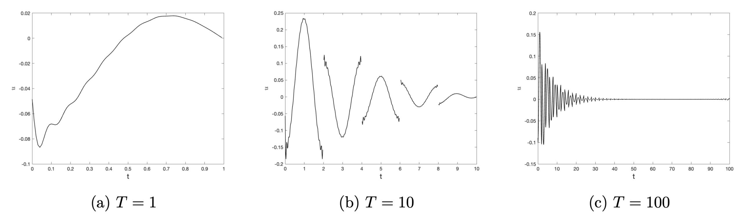
Figure 1. Optimal control u(t) for different values of T  

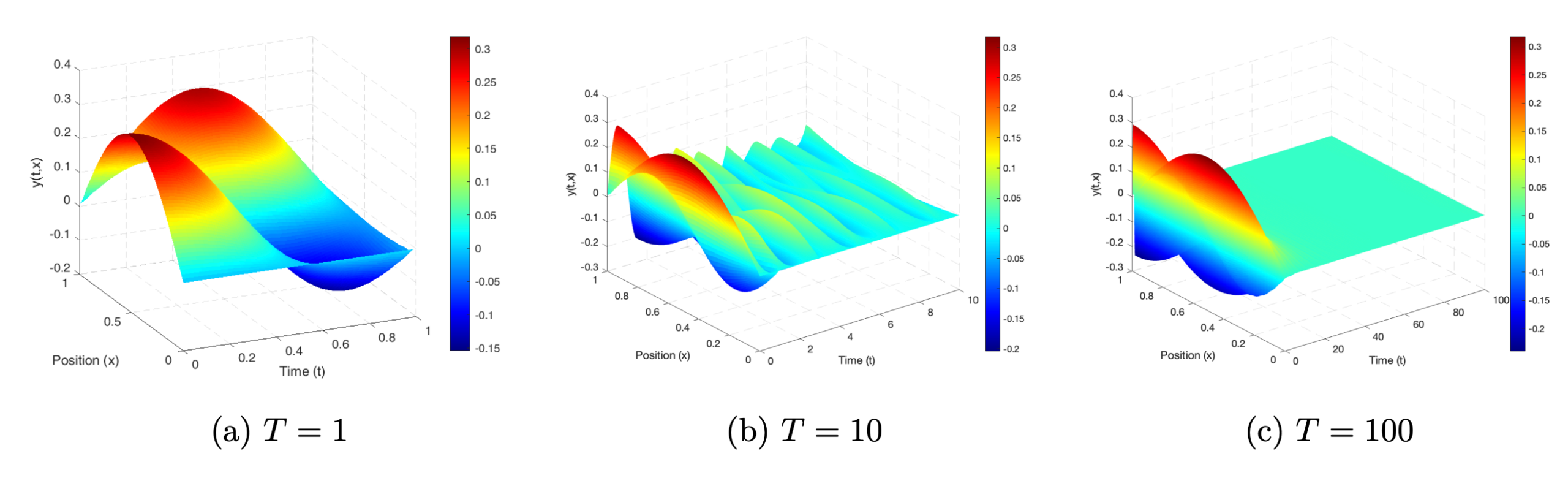
Figure 2. Optimal state y(t,x) for different values of T  

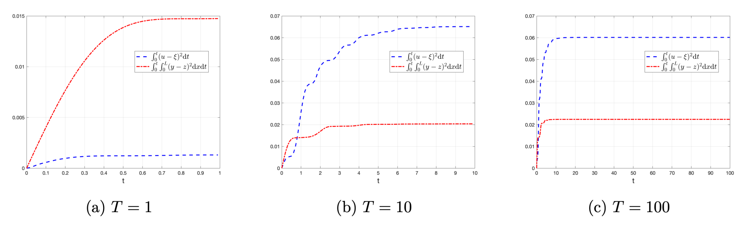
Figure 3. Optimal \int_0^t (u-\xi)^2 {\rm d}t and \int_0^t \int_0^L (y-z)^2 {\rm d}x {\rm d}t for different values of T

 

4 Conclusion

This poster presents the turnpike property and related control aspects. Due to space limitations, details on shape and topology optimization are omitted; for these, please refer to the full paper. The properties of shape and topology optimization problems on networks modeled by graphs are also explored. For the tree network, we show the exponential turnpike property for the wave equation and consider the geometric shape optimization. The new case is the tree with small cycles. In such a case, the topology of optimal network is determined by using the topological derivatives obtained in the static case.

This work was supported by Deutsche Forschungsgemeinschaft (DFG) in the Collaborative Research Centre CRC/Transregio 154, Mathematical Modelling, Simulation and Optimization Using the Example of Gas Networks, Projects C03 and C05, Projektnr. 239904186.

 

5 References

[1] Avdonin, S., Edward, J., Leugering, G. (2023) Controllability for the wave equation on graph with cycle and delta-prime vertex conditions. Evol. Equ. Control Theory 12(6), 1542–1558
[2] Cagnol, J., Zolésio, J.-P. (2022) Hidden shape derivative in the wave equation. In: Systems Modelling and Optimization, Proceedings of the 18th IFIP TC7 Conference, vol. 396, pp. 42–52
[3] Gugat, M., Hante, F.M. (2019) On the turnpike phenomenon for optimal boundary control problems with hyperbolic systems. SIAM J. Control Optim. 57(1), 264–289
[4] Gugat, M. (2015) Optimal Boundary Control and Boundary Stabilization of Hyperbolic Systems. SpringerBriefs in Electrical and Computer Engineering, SpringerBriefs in Control, Automation and Robotics. Springer, Cham
[5] Klarbring, A., Petersson, J., Torstenfelt, B., Karlsson, M. (2003) Topology optimization of flow networks. Computer Methods in Applied Mechanics and Engineering 192(35–36), 3909–3932
[6] Trélat, E., Zhang, C., Zuazua, E. (2018) Steady-state and periodic exponential turnpike property for optimal control problems in Hilbert spaces. SIAM J. Control Optim. 56(2), 1222–1252

  

|| Go to the Math & Research main page

 

You might like!