

Analysis of a local-nonlocal polymer chain model

What does the mathematics of partial differential equations have to do with biology? Of course, one should not be surprised to hear that mathematical equations can be used to model various biological processes. While biologists build such equations, it is the job of mathematicians to ensure that they are well posed, meaning that they admit reasonable solutions and cannot lead to non-physical predictions. In this post, I describe some recent results on the well-posedness of a particular equation modelling the behaviour of polymer chains.
1. The Challenge
Mathematical models of polymer chains are challenging to study because they involve a mixture of local effects and nonlocal effects. This means the behaviour of a polymer chain at one point depends not only on interactions with neighbouring points (local effects), but also with the entire chain (nonlocal effects). There are in fact many examples where nonlocal effects arise. One arises when studying crowd dynamics: on a crowded pavement, a person decides where and how fast to walk based both on their own personal preference (local effects) and on the behaviour of the crowd around them (nonlocal effects).
These mixed local-nonlocal problems pose new challenges compared to purely local problems, which can typically be analyzed using well-established tools from the field of differential equations. The challenge we address in this post is to develop a systematic way to analyze the interplay between local and nonlocal effects in a polymer chain model.
2. Local-nonlocal models of polymer chains
Following [1, 2, 3, 4], we consider a polymer chain of total length T moving inside a bounded domain \Omega\subset\mathbb{R}^{N} (N\ge 1) that contains some fluid. We will assume that this domain has a smooth boundary, denoted by \partial \Omega.
We measure the distance of a point along the chain from one of its ends using a variable t, with t = 0 and t = T being the two opposite ends of the chain. This setup is illustrated in Figure 1.
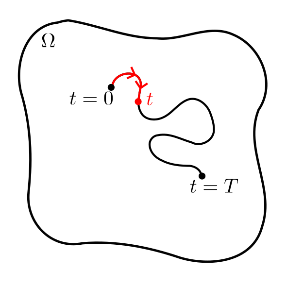
Figure 1. Sketch of a polymer chain (black curved line) of length T in a domain \Omega. The variable t measures the distance from the left endpoint of the chain (t=0).
Let a function u=u(x,t) describe the probability that point t along polymer chain is located at the point x inside the domain \Omega. Suppose we know the probability u(x,0)=u_0(x) that one end of the polymer chain (t=0) is at point x. Then, one can determine u along the entire polymer chain by solving the equations
\begin{cases} \partial_t u +\mathscr{L} u + \displaystyle u\, \varphi\!\left(\int_0^T u(\cdot,\tau)\,\mathrm{d}\tau\right) =0 & in \; Q \coloneqq \Omega\times (0,T),\\ u =0 & on \;\Gamma \coloneqq \partial \Omega \times (0,T),\\ u = 0 & in \; \Sigma \coloneqq (\mathbb{R}^{N}\setminus \Omega)\times (0,T), \\ u(\cdot,0) = u_{0} & in \; \Omega, \qquad (2.1) \end{cases}
where
\mathscr{L} \coloneqq - \Delta + (-\Delta)^{s},\qquad 0\lt s\lt 1. \qquad (2.2)
The operator \Delta is the classical Laplacian, and physically represents the random motion of the polymer chain as it fluctuates through the fluid. For each s\in (0,1), instead, the operator (-\Delta)^s is the fractional Laplace operator and physically represents the effects of possible ‘jumps’ in the location of points along the polymer chain due its sudden reconfiguration. This operator is defined formally by the singular integral
(-\Delta)^s u= \frac{s\,2^{2s}\,\Gamma\left(s + \frac{N}{2}\right)}{\pi^{\frac{N}{2}}\,\Gamma(1-s)} \;\text{P.V.}\int_{\mathbb{R}^{N}}\frac{u(x)-u(y)}{|x-y|^{N+2s}}\;\mathrm{d}y,
where ‘P.V.’ stands for the Cauchy principal value. The nonlocal term \varphi(\int_0^T u \mathrm{d}\tau), instead, appears because each point along the polymer chain produces an energy field around it, hence it interacts with every other point in the chain through a so-called interaction potential \varphi. We will assume that \varphi satisfies the following assumption, which allows for choices of \varphi that are not convex and do not increasing at infinity, like those in Figure 2.
Assumption 2.1.
The potential \varphi:\mathbb{R}\to [0,\infty) is a continuous non-negative function such that \varphi(0)=0 and \tau\mapsto \varphi(\tau)\tau is a non-decreasing differentiable function whose derivative is bounded on every compact subset of \mathbb{R}.
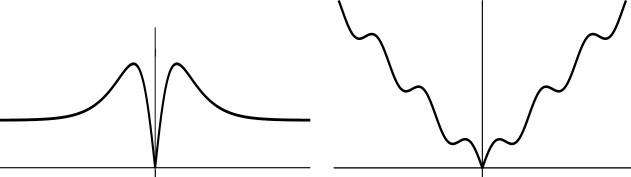
Figure 2. Examples of the potential \varphi (adapted from [2]). Left: \displaystyle \varphi(s)=\frac{2|s|+\sinh|s|}{\cosh|s|}. Right: \varphi(s) = 2|s|+3\sinh|s|.
3. Existence and uniqueness of solutions
Does the polymer chain model described above have well-behaved solutions? Answering this fundamental question is key to ensure the model can be safely used for predicting the behaviour or polymer chains in practice, say through numerical simulations.
Our main contribution is to show that if T is small enough—that is polymer chains are sufficiently short— then yes, ‘nice’ solutions exist. More precisely, we establish the following existence and uniqueness theorem for so-called weak solutions.
Theorem 3.1
Let the probability density u(0,x)=u_0(x) be such that
\|u_{0}\|_{\infty}:= ess \sup_{x \in \Omega} |u_{0}(x)| \lt \infty.
Suppose further that the potential \varphi satisfies Assumption 2.1. Then, for all T>0 problem (2.1) has a weak solution u in the functional space L^\infty(0,T;L^2(\Omega))\cap L^2(0,T;H_0^1(\Omega)). Moreover, this solution is unique for all T small enough that
T^{2} \max_{t\in \left[-T,T\right]}\left|\varphi^{\prime}\left(t\|u_{0}\|_{\infty}\right)\right|\leq \frac{1}{\|u_{0}\|_{\infty}}.
4. A sketch of the proof
The proof of Theorem 3.1 is too technical to be reported in full, but follows an interesting strategy that we outline here without being too precise.
The main idea is to apply the Tikhonoff theorem on the existence of a fixed point of a certain map. To construct this map, we follow [2,3] and consider the following two simplified problems.
4.1. A mixed local-nonlocal elliptic problem.
The first simplified problem is an elliptic local-nonlocal problem, which given a measurable function f:\Omega\to \mathbb{R} asks one to find a function v:\mathbb{R}^N\to \mathbb{R} satisfying
\begin{cases} - \Delta v + (-\Delta)^{s}v + \varphi(v)\,v= f & in \; \Omega,\\ v =0 & on \; \mathbb{R}^{N}\setminus \Omega. \qquad (4.1) \end{cases}
Heuristically, this problem is obtained by integrating the model (2.1) with respect to t from 0 to T. In a sense, the functions v and f correspond to \int_0^T u(\cdot,t)\, dt and u_0-u(\cdot,T), respectively.
A function v in the usual Sobolev space H^{1}_{0}(\Omega) is said to be a weak solution of problem (4.1) if v\varphi(v) is square integrable and
(\nabla v(x), \nabla \psi(x) ) +\frac{C_{N,s}}{2} \iint_{\mathbb{R}^{N}} \frac{(v(x)-v(y))(\psi(x)-\psi(y))}{|x-y|^{N+2 s}} \mathrm{d}y\; \mathrm{d}x +(v\varphi(v),\psi)=(f,\psi) \qquad (4.2)
for all \psi\in H^{1}_{0}(\Omega).
Here, (f,g) = \int f g \, dx stands for the usual L^2 inner product.
If Assumption (2.1) holds and the function f is square integrable on \Omega, then problem (4.1) has a unique weak solution v in the usual Sobolev space H^{1}_{0}(\Omega). This can be proved using the Galerkin method, which first projects the problem onto spaces of finite dimension d where existence and uniqueness are readily established, and then considers the limit as d increases to infinity.
4.2. A mixed local-nonlocal parabolic problem
The second simplified problem is a mixed local-nonlocal linear parabolic problem describing the evolution of an ‘ideal’ polymer chain. It reads
\begin{cases} \partial_t u +\mathscr{L} u + \zeta u=0 & in \; Q,\\ u = 0 & in \; \Sigma , \\ u(\cdot,0) = u_{0}, & in \; \Omega, \qquad (4.3) \end{cases}
where the initial probability u_0 and the bounded potential \zeta are both positive and square-integrable. Using the standard Galerkin method, one can easily obtain a weak solution u for this simplified model in the usual functional space L^2\big(0,T;H^{1}_{0}(\Omega) \cap L^2(\Omega,\zeta)\big), where L^2(\Omega,\zeta) is the Hilbert space with the norm
\|u\|_{L^2(\Omega, \zeta)}^2=\int_\Omega |u(x)|^2\,\zeta(x) dx.
4.3. Combining the two simplified problems
Existence results for the two simplified problems can, with a little work, be combined to establish the existence of weak solutions to our original model (2.1). To do this, we use the so-called the Tychonoff fixed-point theorem, which is a well-known and powerful tool to prove the existence of solutions to partial differential equations.
Tychonoff’s theorem tells us that if a map \pi: Z \to Z from a space Z to itself has certain properties, then it has a fixed point—that is, there exists an element z\in Z such that \pi(z)=Z. For our problem, the right choice of \pi comes from composing the map \zeta \mapsto \mathscr{U}_T(\zeta) from a potential \xi to the corresponding solution of the parabolic problem (4.3) with the map f \mapsto \mathscr{V}(f) from a function f to the corresponding solution of the elliptic problem (4.1). Precisely, we can prove the following result.
Theorem 4.1.
Let T>0 and let u_0 be a square-integrable function. The map w \mapsto \pi(w) := \mathscr{U}_T\left( \varphi( \mathscr{V}(u_0-w)) \right) has a fixed point u_T, that is, u_T = \pi(u_T). Moreover, u_T is a weak solution of problem (2.1).
This theorem already establishes the existence of a solution to our polymer chain model for chains of arbitrary length T. To obtain Theorem 3.1, which is our main result, we therefore only need to establish the uniqueness of these solutions. This can be done if T satisfies the smallness condition in the statement of that theorem using standard calculations based on the so-called “maximum principle”.
5. A look ahead
The results described in this post are a first step towards establishing the well-posedness of the polymer chain model (2.1). However, there are still some challenges to be resolved. First and foremost, our result only applies to sufficiently short polymer chains (that is, small enough T). Our future work will try to remove this restriction. We also plan to investigate the problem of controlling the behaviour of polymer chains and the possible emergence of so-called \emph{turnpike phenomena} in such control problems.
References
[1] Victor N. Starovoitov and B N Starovoitova. Modeling the dynamics of polymer chains in water solution. Application to sensor design. J. Phys.: Conf. Ser., 894 012088.
[2] Victor N. Starovoitov. Boundary value problem for a global-in-time parabolic equation. Math. Methods Appl. Sci., 44(1):1118-1126, 2021.
[3] J-D. Djida and Guy F. Foghem Gounoue and Yannick Kouakep Tchaptchie. Nonlocal complement value problem for a global in time parabolic equation. J. Elliptic. Parabol Equ., 8: 767-789, 2022.
[4] J-D. Djida and G. Mophou and M. Warma. Optimal control of mixed local-nonlocal parabolic PDE with singular boundaryexterior data. Evolution Equations and Control Theory, 11(6): 2129-2163, 2022.
|| Go to the Math & Research main page


