Model-based optimization of ripening processes with feedback modules

1 Important remark

This contribution presents a proof of concept together with numerical results to obtain a first idea how to deal with specific process chains within chemical engineering. The main reference of this webpage entry is [1]. Furthermore, for a first mathematical introduction to nonlocal population balance equations (PBEs) and to a further connection to chemical engineering, feel free to check the related posts which can be found at: Math & Research or check my FAU CAA-AvH profile.

2 Nonlocal PBEs in process chains

The quality of particulate products depends of the process conditions during the synthesis of the particles. It turns out that in several relevant processes the particle size highly determines the efficacy of the final product. The evolution of particle size can be described by nonlocal PBEs. Moreover, the reaction plants often contain recycle streams. A general scheme of the considered application can be seen in Fig. 1. The corresponding feedback rates can be controlled over time which have a significant impact on the whole synthesis. Since also required energy and resources affect the choice of process conditions, the following question arises:

How to choose suitable process conditions such that the produced particles fulfill desired properties?

To answer this, a model-based optimization scheme is presented which describes particle synthesis based on nonlocal PBEs incorporating feedback modules.

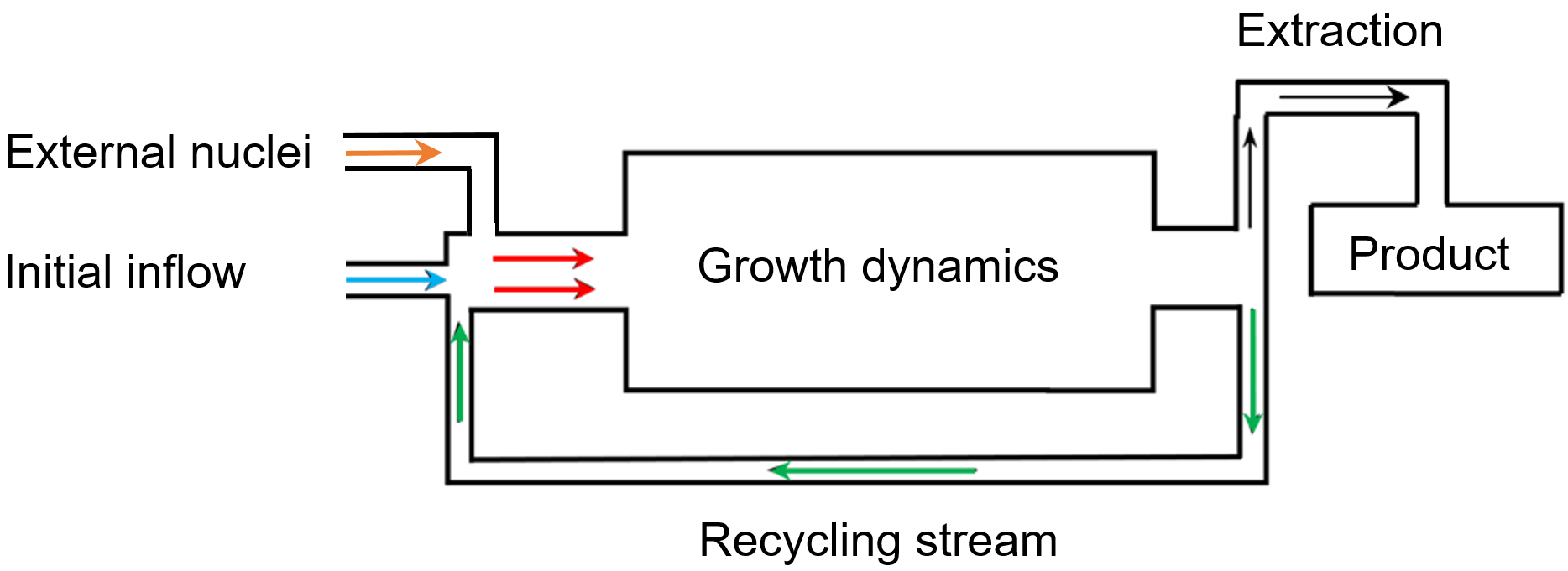
Figure 1. Graphical illustration of a general process chain with recycling stream. The inflow of external nuclei and the rate of the particles fed back into the reactor can be adjusted over time (cf. [1]).

3 Illustration of the concept: Nanoparticle synthesis and minimization of standard deviation

3.1 Mathematical formulation

Now, the general process with feedback modules is illustrated by means of a concrete synthesis process of spherical nanoparticles in which the produced particles can flow back into the system over time (cf. Fig. 2). Diffusion limited growth is considered, i.e., that the velocity function $\lambda$ , which here describes the growth behavior of particles, can be represented as $\lambda[w](t,x)=\frac{c_1(c_2-w)}{x}$ for some real constants $c_1,c_2$ . In the following, terms as, e.g., $q_0$ are so-called particle size distributions (PSDs) where $q_0(x)$ , for a given size $x$ , encodes the number of particles with radius $x$ .

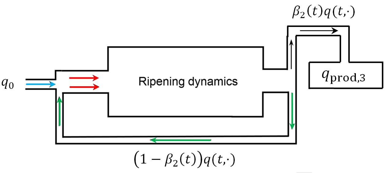
Figure 2. Graphical representation of a general process chain with recycling stream. The PSD of the initial inflow consists of $q_0$ . Over time $(1 -\beta_2(t))q(t,\cdot)$ flows back into the reactor system. The extracted PSD is $\beta_2(t)q(t,\cdot)$ which redounds to the total final product $q_{\textnormal{prod}, 3}$ (cf. [1]).

In this example, the aim is to find a compromise between the following goals by controlling the recycling stream via the time-dependent feedback rate $1-\beta_2$ . Now some required terminology and further explanations of the considered setting together with desired goals:

The initial PSD $q_0$ possesses mean value (in mass-related form) of $2{nm}$
The nonlocal term $W[q](t)$ describes here the total mass of particles in the reactor at time $t$
$U_{\textnormal{ad}}$ describes set of admissible extraction rates $\beta_2$ (admissible controls)
Consider the PSD $q_{\textnormal{prod}, 3}$ of the mass-related product extracted over time
First goal: Reach a given mean diameter $\mu_d=5{nm}$ of $q_{\textnormal{prod}, 3}$
Second goal: Minimize the standard deviation $\sigma = \sigma[q_{\textnormal{prod}, 3} ]$ of $q_{\textnormal{prod}, 3}$ (since one “ultimate” goal would be to produce particles with exactly the same desired size)
Third goal: Minimize the costs of the extraction rate $\beta_2$ . This is analogous to find an optimal feedback rate $1-\beta_2$
$m[q(T,\cdot)]$ describes the mass of the synthesized particles within the reactor at final time
Fourth goal: Minimize $m[q(T,\cdot)]$ (such that there is possible no more reaction material left in the reactor)

This problem can be represented as a so-called optimal control problem: Minimizing a given
cost functional $J [q,\beta_2]$ depending, a.~o., on the solution of a given partial differential equation, here a nonlocal PBE. The various subgoals stated above are contained with corresponding weights in $J[q,\beta_2$ . For final time $T=10{s}$ , the mentioned optimal control problem can be formulated as follows
$\min_{\beta_2\in U_{\textnormal{ad}}} J[q,\beta_2]$

where

$\begin{aligned} J[q,\beta_2]:=(\sigma[q_{\textnormal{prod}, 3}])^2 + 3\cdot 10^{-3} \|\beta_2\|_{L^2((0,T))}^2 + 10^{-3} \|\dot{\beta}_2\|_{L^2((0,T))}^2 + 10^{-2} (m[q(T,\cdot)])^2 \end{aligned}$

such that
$\begin{aligned} q_t(t,x) + \partial_x \left(\frac{5\cdot 10^{-3}(600-W_q(t))}{\max\{x,0.1\}}q(t,x)\right) &= -\beta_2(t)q(t,x) \\ W[q](t) &= \int_{x_{\min}}^\infty \tfrac{4}{3}\pi y^3 q(t,y) dy\\ q_{\textnormal{prod}, 3}(x)& = \int_0^T \beta_2(t)x^3q(t,x) dt \\ \mu &= \mu_d = 5{nm} \end{aligned}$

with

$U_{\textnormal{ad}}:=\{\beta_2 ~:~ \beta_2(t)\in [0,1] \quad \forall t\in[0,T]\}.$

3.2 Numerical results

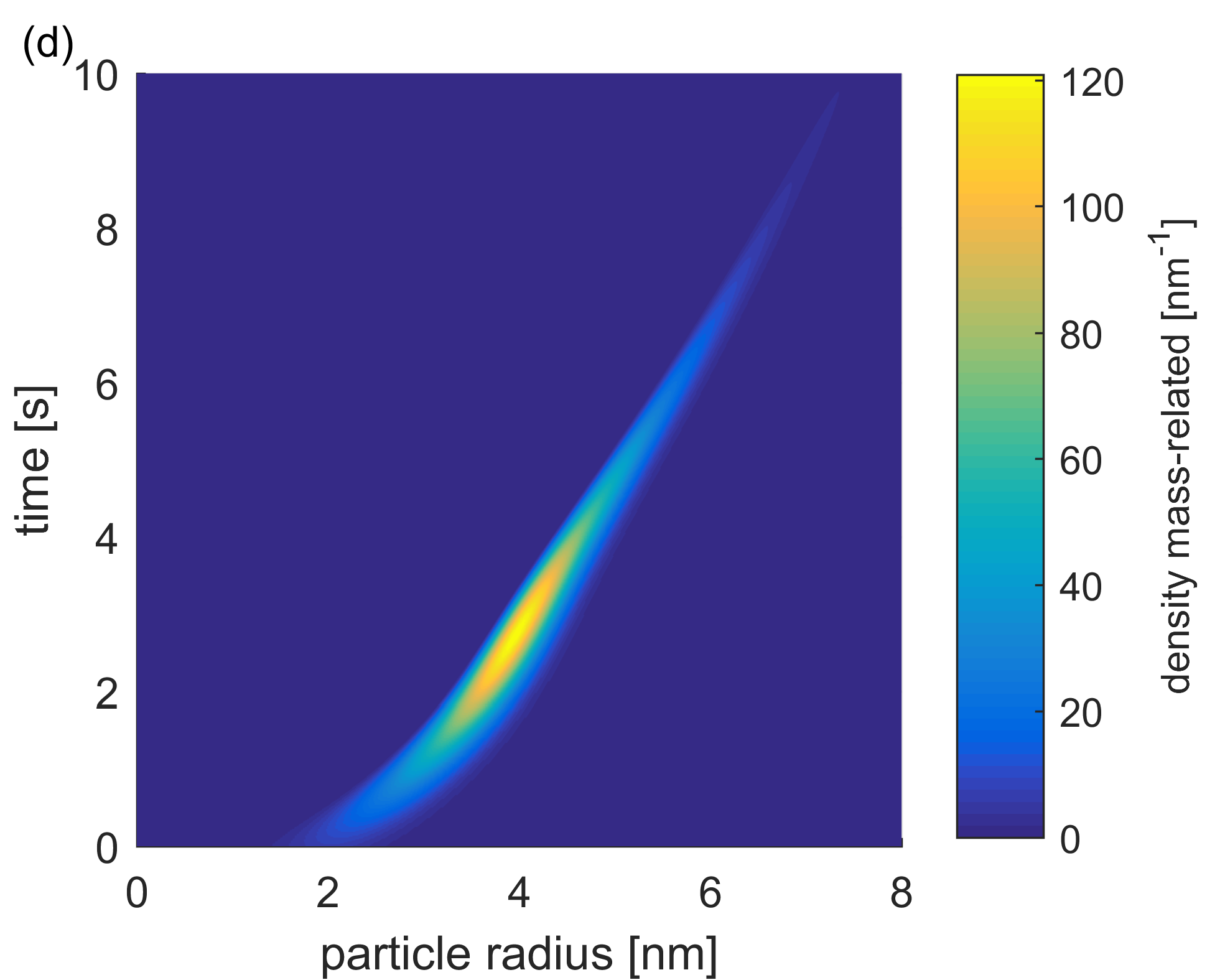
Figs. 3 and 4 show the results of the optimization for a different amount $n_{\beta_2}$ of discretization points of the extraction rate $\beta_2$ . E. g., $n_{\beta_2}=1$ means that only constant controls are considered. Fig. 3 shows, a.~o., that by increasing $n_{\beta_2}$ , i.e. allowing $\beta_2$ to vary more over time, the cost functional decreases by approximately $29{\%}$ and $\sigma$ by approximately $33{\%}$ compared to the constant optimization.

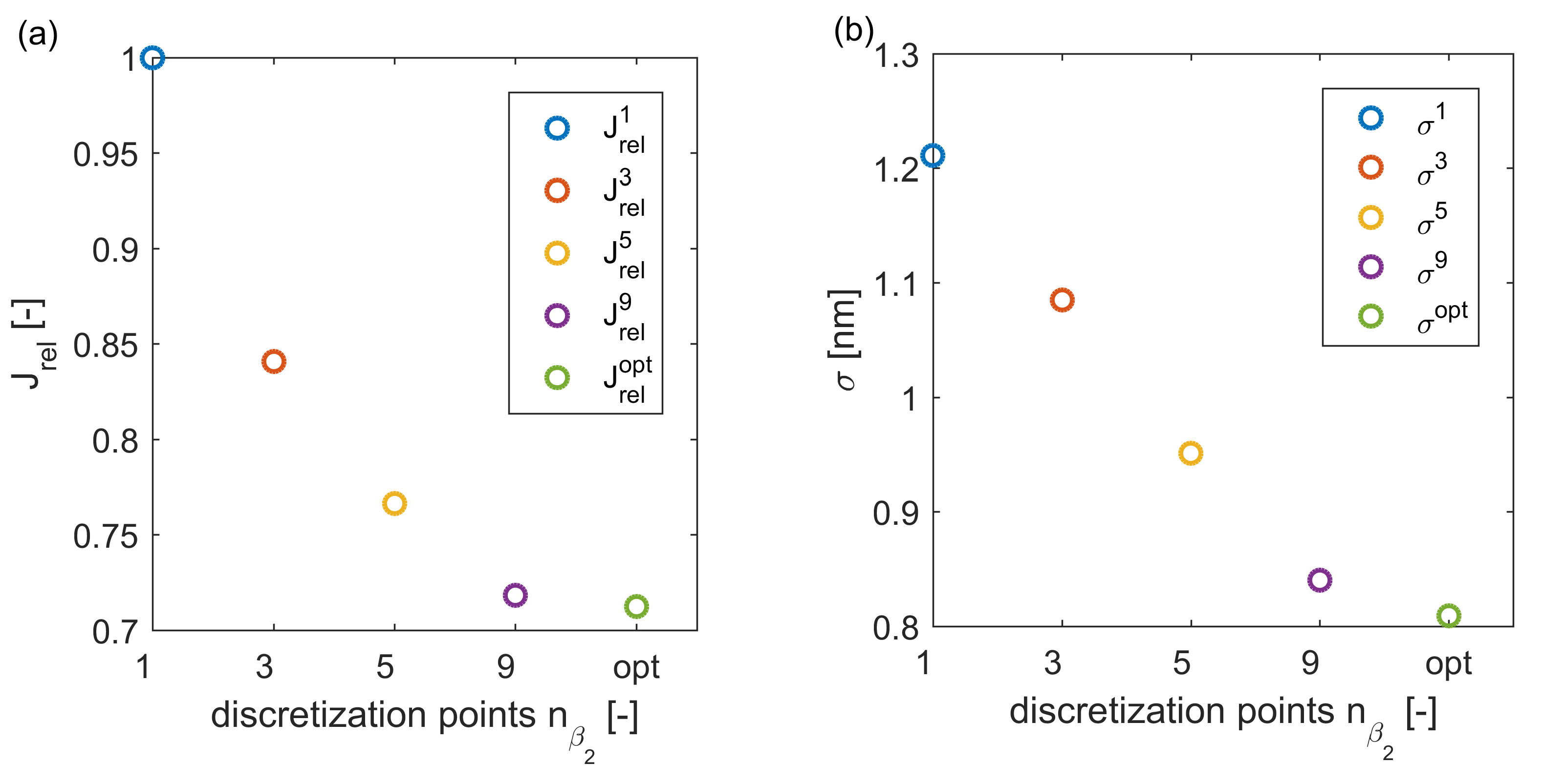
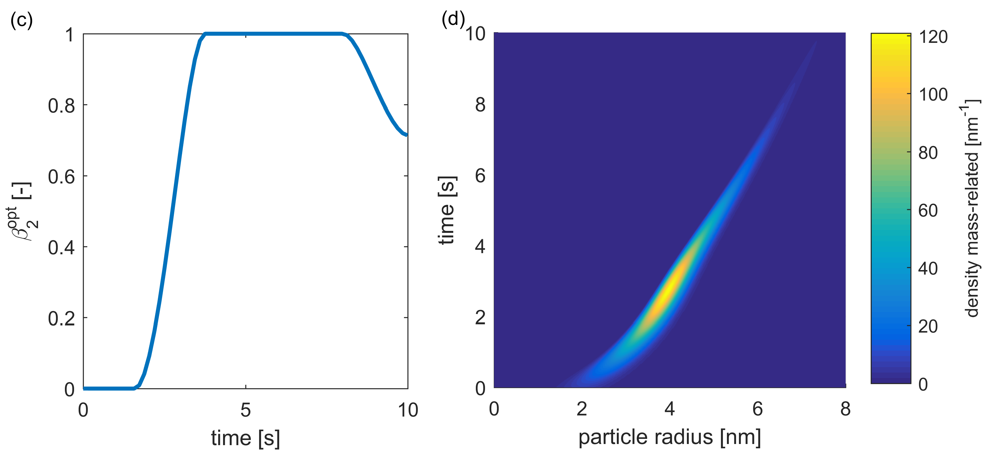
Figure 3. Optimization results: (a) reduction of $J_{\textnormal{rel}}$ ( $J$ normalized) for higher $n_{\beta_2}$ (“opt” for the optimal solution), (b) reduction of $\sigma$ , (c) optimal extraction rate, (d) development of the PSD within the reactor over time

Fig 4 shows the plots of the mass-related number density $q_{0,3}$ of $q_0$ and of the resulting (rescaled) $q_{\textnormal{prod}, 3}$ for different $n_{\beta_2}$ . $\mu_d$ is reached for every optimization and $\sigma$ was decreased after enlarging $n_{\beta_2}$ .

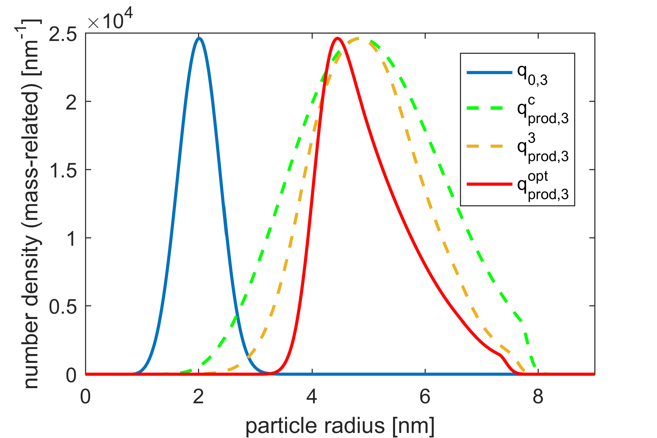
Figure 4. Plots of (rescaled) mass-related initial PSD $q_0$ and the optimal total product $q_{\textnormal{prod}, 3}^{\textnormal{opt}}$ . The dashed curves are generated for $n_{\beta_2}\in\{1,3\}$ . (cf. [1]).

Remark: The outcome of the optimization highly depends on the different weights for the different subgoals in the cost functional. The choice of the weights has to be set in agreement with the considered application.

Final Conclusions

Finally, all optimization goals were achieved and, as also demonstrated in Figs. 3 and 4, it resembles the importance of time-varying process conditions with a large number of discretization points, showing their potential in mechanical process engineering and particle technology. Further material regarding gradient-based optimization schemes, improving efficiency by adjoint calculus and further applications can be found in [1].

References

[1] Spinola, M., Keimer, A., Segets, D., Leugering, G., and Pflug, L. Model-based optimization of ripening processes with feedback modules. In: Chem. Eng. Technol. 43 (2020), pp. 896–903.