PINNs Introductory Code for the Heat Equation

This repository provides some basic insights on Physics Informed Neural Networks (PINNs) and their implementation.

PINNs are numerical methods based on the universal approximation capacity of neural networks, aiming to approximate solutions of partial differential equations. Recently, extensive focus has been on approximating solutions of various equations, leading to the introduction of different PINN concepts. See PINN papers for a walkthrough of the classical literature on PINNs.

GitHub Repository

This repository will show how to solve the 1D heat equation using PINNs.
Resources available at our FAU DCN-AvH GitHub, at: https://github.com/DCN-FAU-AvH/pinns_heat.
This code can be easily modified to solve various equations in higher-dimensional domains.

How PINNs Work for the Heat Equation

Let us consider the heat equation

$\begin{cases}\partial_t u-\partial_{xx} u=f & \text{in }(0,L)\times (0,T),\qquad \text{(PDE)} \\ u(0,t)=u(L,t)=0 &\text{on }(0,T), \qquad\qquad \text{(Boundary conditions)} \\ u(x,0)=u_0(x) &\text{on }(0,L), \qquad\qquad \text{(Initial condition)}\end{cases}$

where $u_0\in L^2(0,L)$ in the initial condition and $f\in L^2(0,T;0,L)$ is a source term. Here, $x$ and $t$ denote the spatial and temporal variables.
We consider a dataset $D=\{d^k\}^{N}_{k=1}$ where $d_k=(x_k,t_k)$ for every $k$ , i.e., a spatial-temporal mesh. We also consider the neural network

${z}^k_{j+1}=\sigma({a}_{j} {z}^{k}_{j}+{b}_j), \quad j\in \{1,\dots,M\},\quad {z}^{k}_{0}={d}^{k},$

with $\sigma$ being the hyperbolic tangent function and $\Theta=\{(a_j,b_j)\}_{j=1}^{M}$ the neural network parameters. We denote by $z_{\Theta}[d^k]$ the neural network output for the data $d^k$ with the parameters $\Theta$ .

PINNs aim to find the parameters $\Theta=\{(a_j,b_j)\}_{j=1}^{M}$ such that

$z_\Theta^k\approx u(x_k,t_k), \quad \text{for every } k\in \{1,\dots, N\} \qquad (1).$

Remark 1
Both the architecture and the activation function of the previous neural network can be changed, taking care that this new architecture has reasonable approximation properties and that the activation function is as differentiable as the PINN scheme requires. In the case of the heat equation, from the standard theory of parabolic equations, the solution is in $C(0,T;L^2(0,L))$ . Therefore, it is enough that the neural network approximates a dense family in $C(0,T;L^2(0,L))$ . It is also necessary to consider a twice-differentiable activation function.

To satisfy (1), the main idea of PINNs is to introduce a penalty to the neural network so that it satisfies both the PDE and the boundary and initial conditions. For this, we introduce the following loss functions.

$Loss_{PDE}(\Theta):= \frac{1}{N_f} \sum_{d^k\in D_{PDE}}^{N_f}\|(\partial_t z_\Theta-\partial_{xx} z_{\Theta})[d^k] - f\|^2,$

$Loss_{BC} (\Theta):= \frac{1}{N_{bc}} \sum_{d^k\in D_{bc}}^{N_{bc}} \| z_{\Theta}[d^k]\|^2, \\$

$Loss_{INT} (\Theta):= \sum_{d^k\in D_0} \|z_{\Theta}[d^k]\|^2,$

where $D_{INT}$ is the set of points of $D$ inside $(0,L)\times(0,T)$ , $D_{BC}$ the set of points of $D$ in $(\{0\}\cup \{L\})\times(0,T)$ and $D_{0}$ the set of points of $D$ in $(0,L)\times\{0\}$ . Thus, the loss function we consider in training the neural network is:

$Loss(\Theta):=w_{PDE}\cdot Loss_{PDE}(\Theta)+w_{BC}\cdot Loss_{BC} (\Theta)+w_{INT}\cdot Loss_{INT} (\Theta),\qquad (2)$

where the constants $w_{PDE}$ , $w_{BC}$ and $w_{INT}$ are hyperparameters of the model.

Remark 2
One of the important advantages of PINNs is that it is not necessary to have labels, as is typically the case in supervised learning. It is sufficient to have a sample of points from our spatio-temporal domain.

Examples in the code

This code contains two examples.
Example_1: This corresponds to the solution of the heat equation on the domain $(x,t) \in (-1,1) \times (0,1)$ .
To illustrate the performance, we chose an exact solution given by $u_{real}^1(x,t) = e^{-t}\sin(\pi x)$ . The source term and the initial condition are chosen to ensure $u_{real}^1$ as a solution of the heat equation.

Example_2: This corresponds to the solution of the heat equation on the domain $(x,t) \in (0,1) \times (0,10)$ .
To illustrate the performance, we chose an exact solution given by $u_{real}^2(x,t) = x^2(x-1)^2(t-1/2)^2$ . The source term and the initial condition are chosen to ensure $u_{real}^2$ as a solution of the heat equation.

Explanation of the code

The code is divided into seven sections:

1. Libraries
We load the libraries that will be used in the main code, including Torch, Numpy, os, deepxde, and matplotlib.

2. Device configuration
General configurations. We define the device and the type of float that will be used in Torch.

3. Tuning Parameters
Here we can tunning the parameters, among them are:
• step: Corresponds to the number of steps in the neural network training process.
• batch_size: To optimize the database, we divide it into batches, and this parameter defines the size of the batches.
• w_bc: These parameters correspond to those introduced in (2).
• w_pde: These parameters correspond to those introduced in (2).
• lr: Learning rate for stochastic gradient descent.
• layers: Corresponds to a vector that represents the architecture of the fully connected neural network. The i-th entry of the vector corresponds to the number of neurons in the i-th layer.
• case: In our code, we have implemented two examples for the heat equation. Therefore, this parameter can take the values example_1 or example_2. Each example has a different domain and source function.
• N_test_x: Number of testing points in space.
• N_test_t: Number of testing points in time.
• N_train_x: Number of training points in space.
• N_train_t: Number of training points in time.
• N_bc: Number of training points on the boundary.

4. Generate data
In this section, we use functions from the data_gen module.
This module allows us to generate data within the domain and at its boundary.
For this, the functions used are:
• get_PDE_dataset: Generates the training data within the domain. It is possible to use Latin hypercube instead of the get_PDE_dataset function.
• get_BC_dataset: Generates training data on the boundary.
• get_test_dataset: Generates testing data.

5. Create Model and Optimizer
We use the FCN module to create the fully connected neural network.
This module contains the following functions:
• Forward: Corresponds to the forward step of the neural network.
• lossBC: Calculates the loss function on the boundary and for the initial condition.
• lossPDE: Calculates the loss function within the domain.
• loss: Corresponds to the sum of lossBC and lossPDE.
• relative_error_l2_norm: Calculates the relative error in the $L^2$ norm. This function is used to compare the testing data and the obtained solution.
• Closure: This function is only used in the case that the chosen optimization method is L-BFGS. The optimizer is also defined. By default, we have selected the ADAM optimizer. It is also possible to use the L-BFGS optimizer (You need to uncomment).

6. Training process
In the training process, we iterate over each batch and over all the data in each batch.
The batches are selected randomly but without repetition.
In each iteration of the training process, the solution with the current parameters is saved, as well as the relative error concerning the real solution.
Images are also generated with this information.

7. Animation
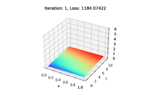
Using the generate_gif function, we create a .gifs and a .mp4 with images of the training process, illustrating how the solution converges to the real one.